Essentials of Machine Learning Algorithms

Introduction

Categories

• supervised learning (predict a specific quantity using training examples with labels)
  • classification
  • regression
• unsupervised learning (look for patterns in the data and doesn’t require labeled data)
  • clustering

• reinforcement learning

• Generative

  • model p(x|y) and then transform it into p(y|x) by applying Bayes rule
  • can be used for unsupervised learning
  • good at handling missing value or detecting outliers ?
• Discriminative
  • model p(y|x) directly
  • doesn't require strong assumption
  • learn decision boundary between classes

Input

The first step of any machine learning method is to represent an instance as an unordered bag of features (i.e. a set of attribute value pairs).

There are 3 types of attributes. Compared with categorical attributes (e.g. yellow, blue, green, red), ordinal attributes (e.g. poor, satisfactory, good, excellent) have a natural ordering and are meaningful to compare. So, one-hot encoding may be required to convert a categorical integer feature into several binary columns, each for one category. Numeric attributes (e.g. 1, -3.14, 2e-3) can be added or multiplied. They are usually normalized to have unit variance or be in the range of [0, 1].

The representation of each datapoint is critical for the performance of machine learning algorithms. The process of picking attributes is also called feature engining.

When it comes to images, text and time series, attributes are not obvious.

For handwritten digits recognition, each pixel can be used as a separate attribute because the same pixel has the same meaning after each digit being isolated, rescaled and de-slanted. As for recognizing an object in an image, using pixels as attributes doesn’t work. A possible approach is to segment the image into regions and then extract features describing the region.

Bag-of-words (sparse vector in implementation) combined with naive bayes classifier is commonly used for text classification, such as spam detection and topic identification.

Music (a kind of time series data) can be decomposed by Fourier transformation into a sum of sine waves of different frequencies and then attribute values are weights of different base frequencies. This representation is insensitive to shift and volume.

Evaluation

It's easy to be perfect on training data while hard to do well on future data. Overfitting means the predictor is too complex or flexible and fit noise while underfitting means the predictor is too simplistic or rigid to capture salient patterns in the data.

Most machine learning algorithms have hyperparameters to control the flexibility. They should be tuned to minimize generalization error.

Generalization error measures how well the predictor behaves on future data. Testing error is an estimate of the true generalization error.

The common methodology of evaluating a model is as follows:

• training set: train/fit the model
• validation set: pick best performing algorithm, fine-tune parameters
• test set: estimate future error

A better way is Cross validation especially when training examples are very limited

1. Randomly split the data into N folds. Stratification helps to keep labels balanced in training and test sets.
2. Select each fold for testing in turn and the remaining N-1 folds for training.
3. Average the error or accuracy over N test folds

What metrics do we use to measure how accurate our system is?

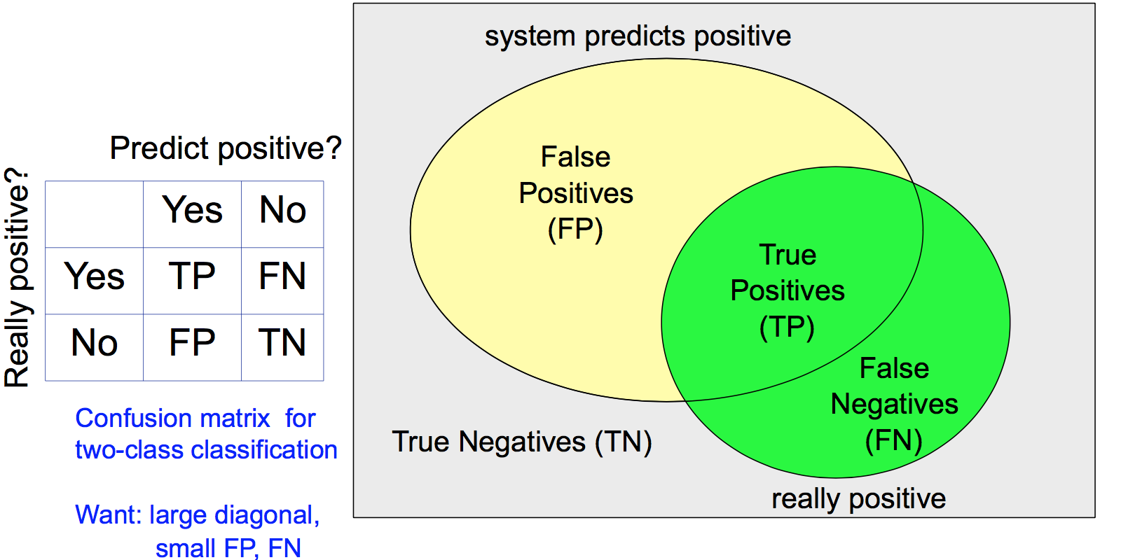
Classification

Accuracy is not enough because it cannot handle unbalanced classes. For example, we are predicting whether an earthquake is about to happen. A predictor which always says no will have very high accuracy but doesn't help.

More measures are needed:

1. False alarm rate (FPR) and miss rate (1-TPR)
2. Precision $\frac{TP}{TP+FP}$ and recall $\frac{TP}{TP+FN}$, F-measure 2/(1/Recall+1/Precision)
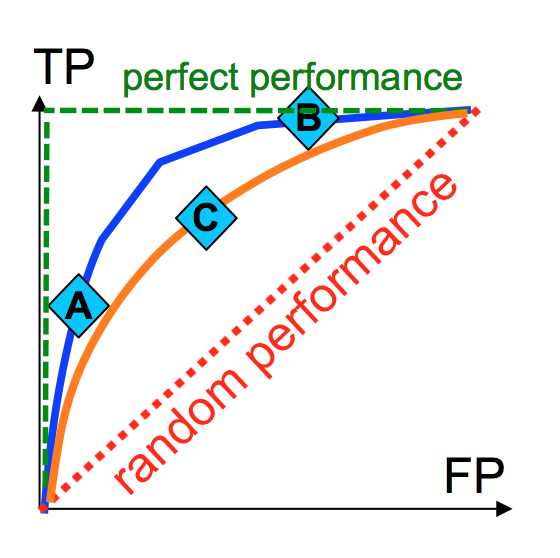
3. ROC curve (TPR/Recall vs FPR $\frac{FP}{FP+TN}$ as threshold varies)

Regression

measure difference between predicted and true values

• Mean Squared Error: very sensitive to outliers
• Mean Absolute Error
• Median Absolute Deviation
• Correlation coefficient for ranking tasks

Naive Bayes

Nauve Bayes predicts class label by applying Bayes rule with independence assumption between features. It's naive because this assumption may not be correct.

$$P(y|x) = \frac{P(x|y)P(y)}{\sum_{y\prime}P(x|y_\prime)P(y_\prime)}$$

• prior $P(y)$
• class model $P(x|y)$
• normalizer $P(x)$

NB makes independence assumption to model $P(x|y)$. Assume attributes $x_1 \cdots x_n$ are conditionally independent give y, i.e $P(x_i|x_1 \cdots x_{i-1}, y) \approx P(x_i|y)$.

$$\begin{align} P(x_1 \cdots x_d |y) & = \prod_{i=1}^{d} P(x_i|x_1 \cdots x_{i-1}, y) \\ & \approx \prod_{i=1}^{d} P(x_i|y) \end{align}$$

There are 2 types of NB classifiers.

• discrete case Multinomial Naive Bayes (i.e. $P(x_i|y)$ is estimated by computing frequency of an attribute value within each class)
• continuous case Gaussian Naive Bayes (i.e. every attribute is normal distribution within each class)

NB has 2 weakness.

1. zero-frequency: smoothing
2. strong assumption

NB can easily handle missing value by just ignoring it for some attribute based on conditional independence assumption between attributes.

Decision Trees

The algorithm used to build decision tree is called ID3:

0. root node contain all the training examples
1. find the best/decision attribute A which produces maximum information gain after split
2. for each value of A, create a child node and split training examples into child nodes
3. stop if the subset in child node is pure otherwise continue split the child node

• Classification: most frequent class in the subset of a leaf
• Regression: average of training examples in the subset

Pros

1. interpretable: human can understand the decisions which make an item positive
2. can handle missing value and irrelevant attribute
3. compact and fast at testing

Cons

1. greedy: may not find the best tree
2. only axis-aligned split of data

Problems

1. Overfitting can be avoided by post-pruning nodes while performance on validation set keeps improving.
2. Information gain is biased towards attributes with many possible values and use GainRatio instead.
3. Continuous attribute can be handled by converting it into discrete attribute using thresholds (binary or multivariate).

RandomForest

1. Grow multiple full (without pruning) decision trees from subsets of training examples
2. Given a new data point X, classify using each of the trees and use majority vote to predict the class

RF is the state-of-art method for many classification tasks.

Linear regression

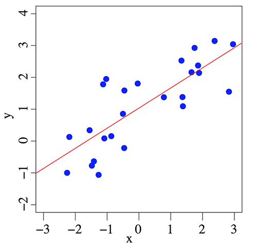
Linear regression assumes y is a linear function of all attributes.

$$f(x,w)=w_0 +w_1x_1 + \cdots +w_Dx_D$$

Fit the data when there is only one feature

With more features, the fitted model forms a plane or hyperplane instead of a line.

Loss function is square error $O(w) = \sum_{i=0}^{n} (y_i - \mathbf{w}_\top \mathbf{x}_i)^2$. To minimize the loss function with respect to parameters W, linear regression has an analytical solution. $$\hat{\pmb{w}} = (\phi^T\phi)^{-1}\phi^T \pmb{y}$$

Always visualize (graphical diagnose) to check:

1. whether there is a linear relationship between input and target or not
2. outliers (linear regression is very sensitive to outliers)

Actually, linear regression is more powerful than you would expect.

Non-linear regression means we transform the original attributes x non-linearly into new attributes $\phi(x)$ (this process is called basic expansion) and then do linear regression.

• polynomial regression transforms an attribute x into $\phi(x) = (1, x, x^2, \cdots, x^M)^T$
• RBF regression uses Gaussians as basis function

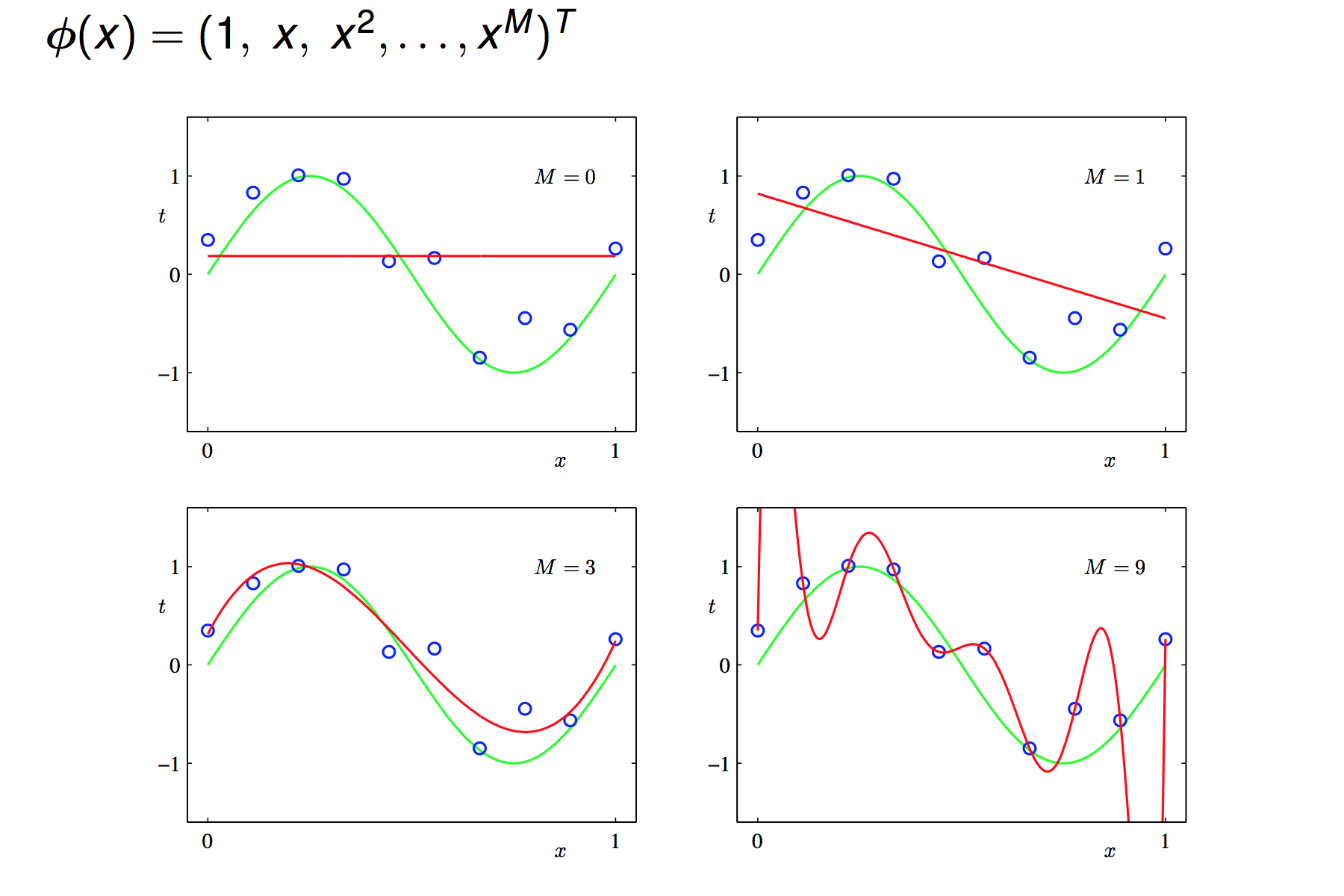
Be careful that too many new features might result in overfitting.

Logistic regression

It's a classifier in fact though the name is quite misleading.

The formula of the decision boundary (a line for 2 features and a hyperplane for higher dimension) is $$f(x,w)=w^T x + w_0$$

As shown in the figure below, the feature space is divided into 2 regions by the decision boundary and each region corresponds to a class.

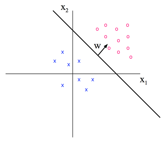
So far it's quite similar to linear regression but notice that the y-axis in the figure above is feature x2 instead of target value y. In a 2 classes case, assuming the red circle represents class 1, y=1 if f(x,w)>0.

In order to model the probability P(y = 1|x), sigmoid/logistics function $\sigma(z)=\frac{1}{(1+exp(−z))}$ is applied to squash f into [0, 1]. $$p(y = 1|x) = \sigma(w^Tx+w_0)$$

• bias parameter $w_0$ shifts the position of the hyperplane
• weight vector $w=(w_1, w_2, \cdots, w_d)^\top$ is the normal vector of the hyperplane (perpendicular)
  • direction of w affects the angle of the hyperplane
  • magnitude of w affects how certain (probability close to 0 or 1) the classification is

Parameters W are determined by maximizing the log likelihood (equivalently, minimizing the negative log likelihood) using numerical optimization algorithm such as gradient descent. Assuming the dataset D is independent and identical distributed, the likelihood of the training data is $$P(D|\mathbf{w}) = \prod_{i=0}^{n}p(y=y_i|\mathbf{x_i}, \mathbf{w})$$

Gradient descent iteratively moves to the minimum of error surface on weight space by subtracting a proportion of the gradient of E with respect to weight parameters. The pseudo code for batch gradient descent is as follows:

initialize w
while E(w) is unacceptably high
    calculate g = ∂E/∂w
    update w = w - ηg
end
return w

Neural networks suffer from local optima. Fortunately, logistic regression has a unique optimum (i.e. the global optima).

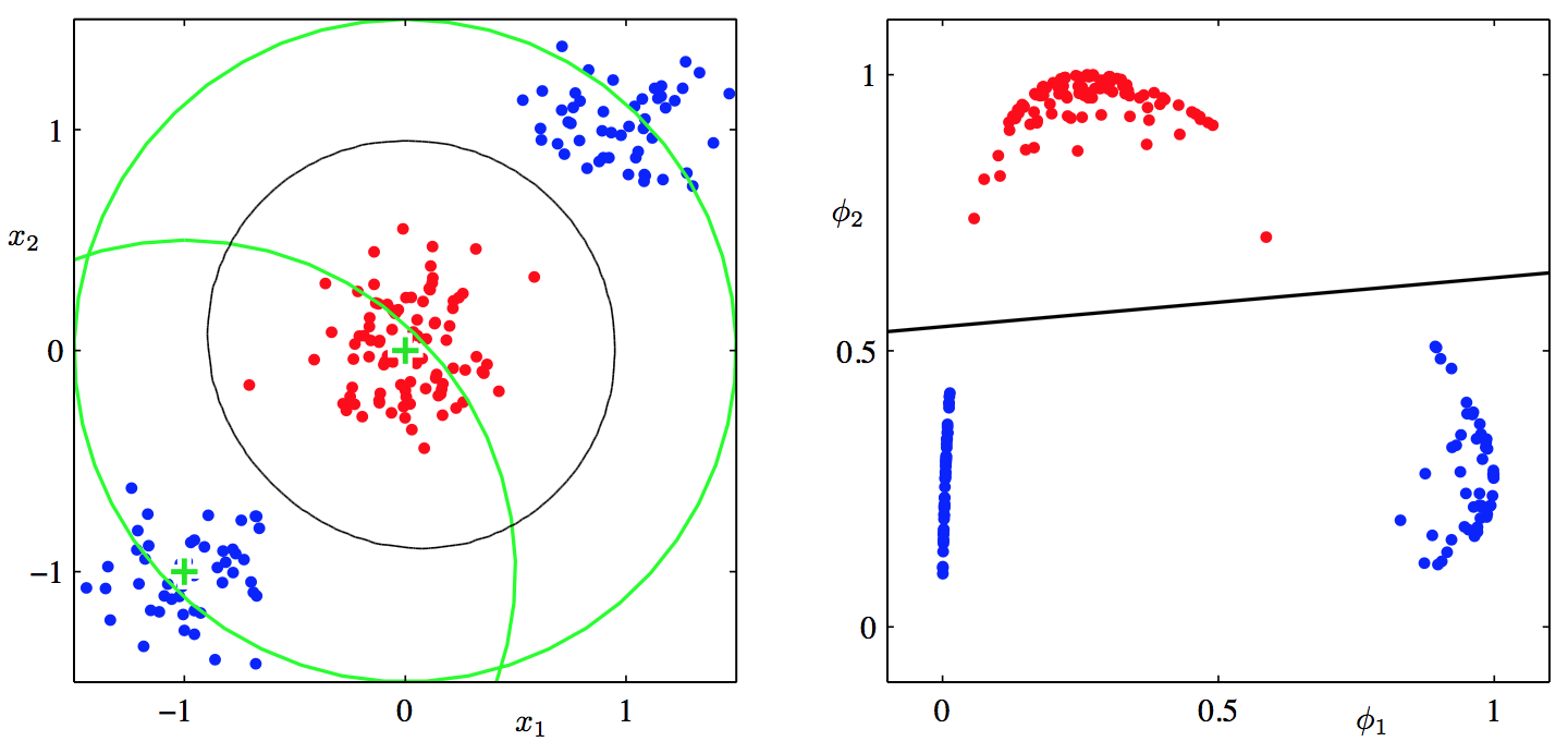
Logistic regression learns a linear decision boundary. In a linearly separable dataset, logistic regression can classify every training example correctly. However, LR cannot get 100% accuracy on a non-linearly separable dataset (e.g. at most 75% accuracy on XOR dataset). Like linear regression, we can apply non-linear transformation to the input space (i.e. attributes X) to make them linearly separable. Here is an example, using two Gaussian basis function, the data in the new feature space is linearly separable.

For multi-class classification, we use a separate weight vector for each class and output the probability using softmax instead of logistic function. $$P(y=k|\mathbf{x}) = \frac{\exp(\mathbf{w}_k^\top \mathbf{x})}{\sum_{j=1}^{C} \exp(\mathbf{w}_j^\top \mathbf{x})}$$

SVM

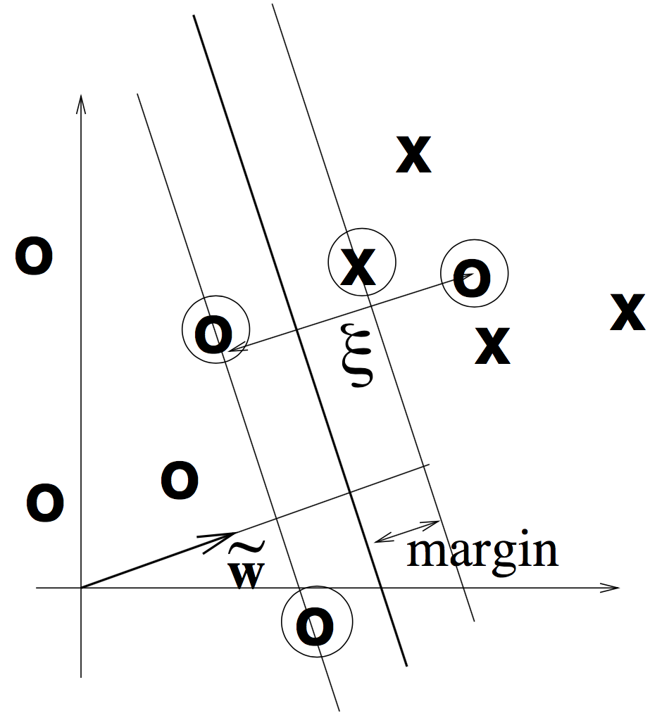
Like logistic regression, Support Vector Machine (SVM) draws a decision boundary or hyperplane $w^Tx + w_0 = 0$ in the feature space but with different objective function. SVM maximizes margin + slack. Margin is the distance from the closest training point to the decision boundary. $\text{margin} = \min_i \frac{1}{||\mathbf{w}||}|\mathbf{w^\top x_i} + w_0|$. slack variable $\xi$ is the distance from a point to its marginal hyperplane. It's introduced to deal with non-separable data but also applicable for a separable data set.

The optimization problem is to minimize $||w||^2 + C(\sum_{i=1}^{n} \xi_i^k)$. The solution looks like $\mathbf{w} = \sum_i \alpha_i y_i \mathbf{x_i}$. The hyperplane is only determined by just a few datapoints (support vectors). Prediction on new data point x is $$\begin{align} f(x) &= \text{sign}[\mathbf{w^\top x} + w_0] \\ &= \text{sign}[\sum_{i=1}^{n} \alpha_i y_i (\mathbf{x_i}^\top \mathbf{x}) + w_0] \end{align}$$

Plain SVM is a linear classifier. Like logistic regression, SVM can also be made non-linear by using basis expansion which is implemented in kernel trick. Non-linear transformation makes data more separable. kernel makes it easier and faster to compute with if the expanded feature space is high dimensional (even infinite). $$k(\mathbf{x}_i, \mathbf{x}_j) = \phi(\mathbf{x}_i)^\top \phi(\mathbf{x}_j)$$ Prediction is now $f(x) = \text{sign}[\sum_{i=1}^{n} \alpha_i y_i k(\mathbf{x_i}, \mathbf{x}) + w_0]$. So, we don't bother to calculate $\phi(\mathbf{x})$. For example, for 2-d input space,

$$\phi(\mathbf{x}_i) = \left( \begin{array}{c} x^2_{i,1} \\ \sqrt{2}x_{i,1}x_{i,2} \\ x^2_{i,2} \end{array} \right)$$ $$k(\mathbf{x}_i, \mathbf{x}_j) = (\mathbf{x}_i^\top \mathbf{x}_j)^2$$

Combined with kernels such as polynomial and RBF, SVM has achieved good empirical results in many tasks.

KNN

K Nearest Neighbors (KNN) uses intuition to predict a new test point X: output the value of the most similar training example. It's simple because it doesn't make assumption about the data and let the data "speak" for itself instead.

KNN method can be used for both classification and regression.

Algorithm

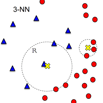
1. compute distance between X and every training example Xi
2. select K closest training instances (neighbors)
3. output the most frequent class label or mean of neighbors

Problems

choosing the value of K

• Too large K will result in everything classified as the most probable class.
• Too small K will make the classification unstable.
• Best practice is to pick K that gives the best performance on a held-out set.

distance measure

The distance defines which examples are similar and which aren't. Common measures are:

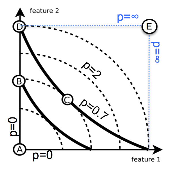
• Minkowski distance (p-term)$D(x, x^\prime) = \sqrt[p]{\sum_{d}{|x_d-x_d^\prime|^p}}$
  • p=2: Euclidian (sensitive to extreme difference in single attribute)
  • p=1: Manhattan
  • p=0: Hamming
• Kullback Leibler divergence $D(x, x^\prime) = -\sum_d x_d\log\frac{x_d}{x_d^\prime}$

ties

What if there are equal number of positive and negative neighbors?

• randomly choose one
• pick class with greater prior across the dataset
• use the nearest or 1-NN classifier to decide (but can still have tie problem)

missing value

A reasonable choice is to fill in with average value of the attribute across entire dataset.

computationally expensive

The naive implementation needs to store all training examples and compare the test point one-by-one to each training example (Complexity is O(nd)). The idea to solve this is to find a small subset of training examples that are potential near neighbors.

• K-D tree
  • use median to split the data repeatedly
  • low-dimensionality, real-valued data
• locality-sensitive hashing
  • use k hyperplane to slice the space into 2^k regions
  • high-d, real-valued
• inverted lists
  • maintain a map from possible attribute values to a list of training examples that contain the value and then merge the lists for attributes present in the testing instance
  • high-d, discrete, sparse

However, both K-D tree and locality-sensitive hashing have the problem of missing neighbors.

K-Means

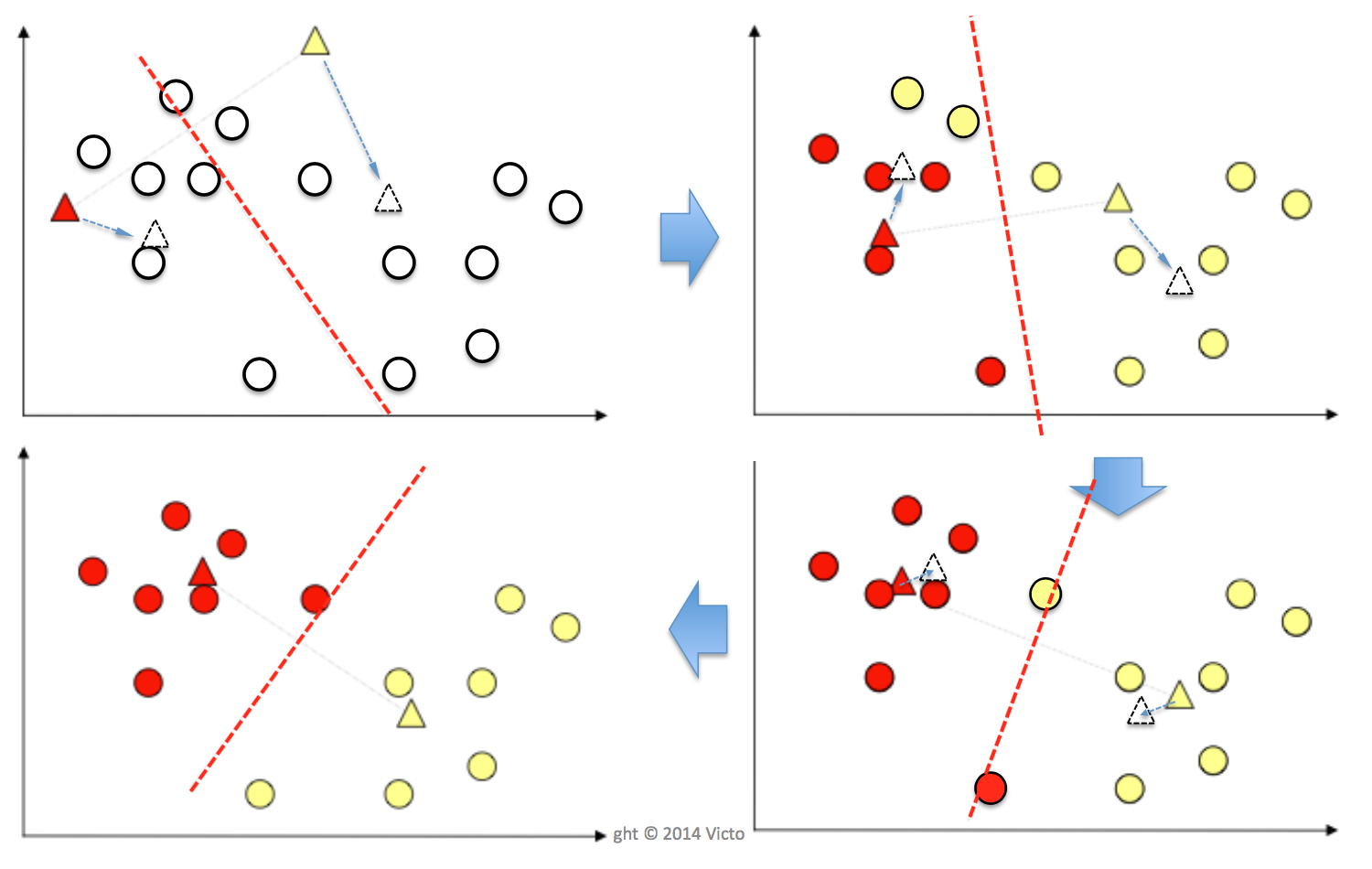
K-Means is an unsupervised clustering algorithm which produces polythetic, hard boundary and flat clusters. K-Means splits data into K sub-population where membership is defined by the distance. The algorithm goes like this:

input K, set of datapoints X1, X2,...,Xn
place K centroids at random locations in the feature space, each corresponding to a cluster
repeat until convergence (i.e. no centroid changes):
    for each datapoint Xi:
        compute the Euclidian distance between Xi and each centroid
        find the closest centroid and assign Xi to the corresponding cluster 
    for each cluster j=1...K:
        update centroid Cj as the mean of all datapoints assigned to cluster j in the previous step

Problems

local minimum

KMeans minimizes the aggregate intra-cluster distance (sum of squared distance between each datapoint and its centroid $\sum_j \sum_{x_i \rightarrow c_j} D(x_i, c_j)^2$) in each iteration until convergence. Different starting points will result in different minima. The solution is to run several times with random starting points and pick clustering that yields the smallest aggregate distance.

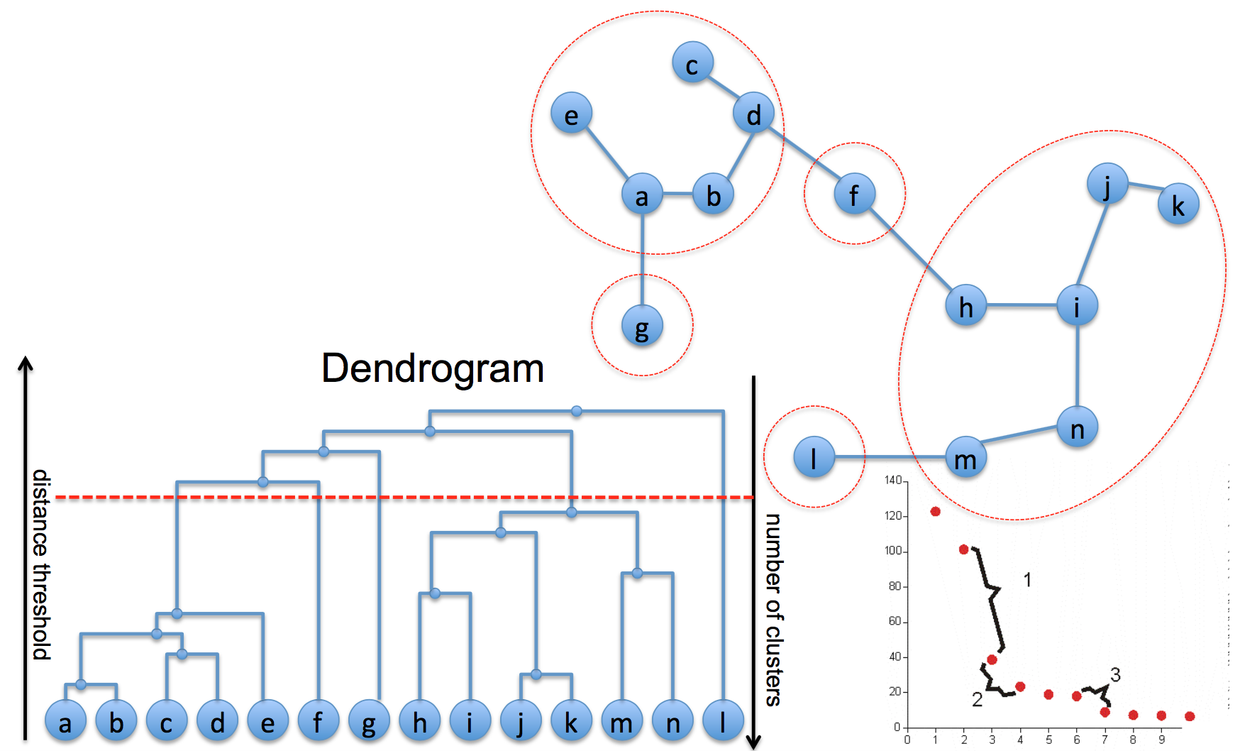
pick K

K must be explicitly specified as the input. We specify K=10 for clustering images of handwritten digits. What if we don't know how many clusters there are in the data? Aggregate distance is monotonically decreasing with K. Usually, we plot the aggregate distance against the value of K (this is called screen plot) and visually pick K where the mountain ends and rubble begins (make aggregate distance decrease the most).

Evaluation

Evaluation for clustering algorithm is not easy. If class labels are available, we need to align clusters with classes before measuring accuracy.

Otherwise, we could sample some pairs and ask human whether they should be in the same group or not. Sample pairs can also be generated from class labels. By counting matching (TP, TN) and non-matching pairs (FP, FN), we can compute accuracy, F1, etc.

Application

Inspired by bag-of-words, an image can be represented by a bag of visual words.

1. divide a large image into small regions/patches (e.g. 10x10)
2. extract appearance features for each patch such as distribution of colors, texture, edge orient
3. use K-Means to cluster feature vectors of all regions across all images in the dataset. As a result, similar regions will end up in the same cluster and have the same cluster id.
4. every region in every image is represented by its cluster label/id. An image is represented in K dimensional visual words.

Mixture Models

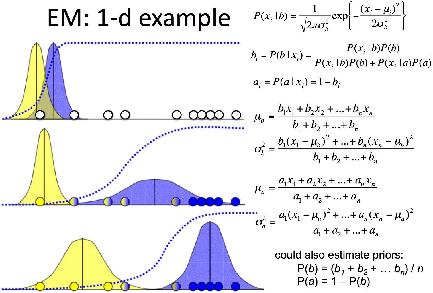
Suppose the distribution of our data (1-d) looks like 2 mixed Gaussian function, Gaussian mixture model can help us automatically discover all parameters for the 2 Gaussian sources.

Mixture model is a probabilistically-grounded way of doing soft clustering. Each cluster follows a Gaussian (continuous) or multinomial (discrete) distribution. Mixture Model is also called expectation maximization because the convergence goal is to maximize the log likelihood of data (expectation).

Assuming the dataset is iid, the likelihood of n training examples under the mixture model of K sources is

$$\begin{align} L = \log{P(x_1\cdots x_n)} &= \log{\prod_{i=1}^{n}P(x_i)} \\ &= \sum_{i=1}^{n}\log{\sum_{k=1}^{K}P(k)P(x_i|k)} \end{align}$$

Let's walk through the 1-d GMM example mentioned above.

1. initiate 2 random Gaussians$(μ_a, σ_a^2), (μ_b, σ_b^2)$ with equal priors p(a) = p(b) = 0.5
2. repeat until convergence
   • E-step: for each point x and each Gaussian $k \in {a, b}$, compute P(k|x) using Bayes rule
   • M-step: adjust $(μ_a, σ_a^2), (μ_b, σ_b^2)$ and priors according to posteriors of all datapoints in the previous step

EM has the same problems as K-Means.

Agglomerative clustering

Agglomerative is a bottom up clustering algorithm which yields a hierarchical tree of clusters.

Given a dataset of n training examples, Agglomerative clustering
1. start with a collection C of n singleton clusters, each containing one datapoint.
2. repeat until only one cluster is left (n-1 iterations)
    1. find the closest pair of clusters ci, cj
    2. merge them into one bigger cluster and update the collection

How do we compute the distance between 2 clusters?

• centroids: distance between centroids of the 2 clusters
• single line: distance between 2 closest points in the 2 cluster $$D(c_1, c_2) = \min_{x_1 \in c_1, x_2 \in c_2}{D(x_1, x_2)}$$
• complete link: distance between 2 furthest points $$D(c_1, c_2) = \max_{x_1 \in c_1, x_2 \in c_2}{D(x_1, x_2)}$$
• average link: average of all pairwise distance $$D(c_1, c_2) = \frac{1}{|c_1|}\frac{1}{|c_2|} \sum_{x_1 \in c_1} \sum_{x_2 \in c_2} D(x_1, x_2)$$
• Ward: total squared distance from the centroid of joint cluster

The distance matrix is updated using Lance-Williams algorithm after merging 2 clusters.

PCA

Principle Components Analysis (PCA) is a dimensionality reduction algorithm.

Datasets are typically high dimensional such as images represented by pixels. True dimensionality is usually much lower than observed dimensionality because there are correlated or redundant features. High dimensional dataset is sparse in the feature space which makes statistics based methods unstable to predict. Dimensionality reduction helps to dramatically reduce the size of data and speedup computation. It also allows estimating probabilities of high-dimensional sparse data.

PCA represents an instance using fewer features which explains the maximum variance in the data.

Given a D-dimensional dataset, PCA computes eigenvectors and their corresponding eigenvalues from covariance matrix. We get D D-dimensional eigenvectors and D eigenvalues. It has been proved that eigenvectors maximize the variance (an eigenvector points to the direction of greatest variability in the data) and eigenvalue is the variance along its eigenvector.

We pick K eigenvectors (they are called principle components) associated with the largest K eigenvalues (variance) as new dimensions.

Given a new instance, we project it to these new dimensions to get a lower (K<<D) dimensional representation. That is, we compute dot product between the new instance and each principle component to get a vector of new coordinates.

Problems

1. pick K: Usually we want to pick the first K eigenvectors which explain 90% of the total variance.
2. Covariance is sensitive to large attribute: normalize each attribute to zero mean and unit variance.
3. PCA assumes the subspace is linear: For example, if we want to reduce from 2D to 1D, the datapoints in the original 2D space should be close to a straight line.
4. Make classes less discriminative: Linear Discriminant Analysis makes it easier to distinguish classes but doesn't guarantee.