Reinforcement Learning Introduction

Richard S. Sutton's "Reinforcement learning: An Introduction, 2nd edition" is a very good textbook for RL but it is too long. This article acts as a highly condensed note for that book.

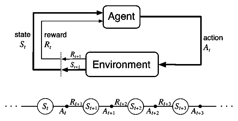
Reinforcement Learning (RL) is a kind of machine learning method which trains an agent to make decisions at a series of discrete time steps (sequential decision problem) via repeated interaction with the environment (trial and error) in order to achieve the maximum return. Given a state which represents all information about the current environment/world, the agent chooses the optimal action and receives a reward. The agent repeats this for next state/time-step.

Multi-Armed bandits

Multi-Armed bandits are non-associative tasks where actions are selected without considering states. They are not full reinforcement learning problem. However, exploration strategy especially ε-Greedy developed in this section is widely used in reinforcement learning algorithms.

bandit problem

A slot machine has k levers. Each action is a play of one of the levers.

The reward of action A can be:

• deterministic or stochastic
  • deterministic: a fixed value
  • stochastic: e.g., selected from a normal distribution with mean $\mu$ and variance $\sigma$
• stationary or non-stationary
  • stationary: parameters are constants
  • non-stationary: parameter such as $\mu$ changes over time

Action value methods

• $q_*(a)$: value of action a is the expected/mean return of action a (selecting some lever).
• goal: maximize the total rewards over some time period
• how: select the action with highest value

Since $q_*(a)$ is unknown, we need to estimate it. Estimate of the value of action a at time step t is $Q_t(a)$. Consider a specific action, let $Q_n$ denote the estimate of the action value after it has been selected $n-1$ times.

sample average: $$Q_n \doteq \frac{R_1 + R_2 +\cdots+R_{n-1}}{n-1}$$

Note: dot over the equal sign means definition

incrementally computed sample average: $$Q_{n+1} = Q_{n} + \frac{1}{n} [R_n - Q_n]$$

For non-stationary problem, assign more weights to recent rewards by using a constant step size $\alpha \in (0, 1]$ (called exponential recency-weighted average). This method doesn't completely converge but is desirable to track the best action over time. $$Q_{n+1} \doteq Q_{n} + \alpha [R_n - Q_n]$$

Estimate Q(a) will converge to true action value $q_*(a)$ if: $$\sum_{n=1}^\infty \alpha_n \to \infty \quad\text{and}\quad \sum_{n=1}^\infty \alpha_n^2 < \infty$$ This is called standard stochastic approximation condition or standard α condition.

"conflict" between exploration and exploitation

There is at least one action whose estimated value is greatest.

• exploiting: select one of these greedy actions
• exploring: select one of the non-greedy actions, enables you to improve your estimate of the non-greedy action’s value, i.e., find better actions

Different methods to balance exploration and exploitation

• ε-Greedy
• Optimistic Initial Values (for stationary problem only): encourage exploration by using optimistic (larger than any possible value) initial values $Q_1(a)$
• Upper Confidence Bound (UCB) action selection: improve ε-Greedy by choosing actions with higher upper bound on action value or, equivalently with preference for actions that have been selected fewer times (with more uncertainty in the action-value estimate). $$A_t \doteq \operatorname*{argmax}_a \left[ Q_t(a) + c\sqrt{\frac{\ln t}{N_t(a)}} \right]$$

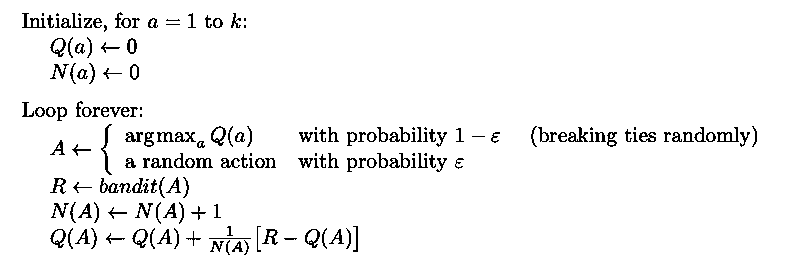
A complete bandit algorithm using incrementally computed sample average and ε-Greedy action selection is shown below:

Gradient methods

Gradient methods use a soft-max distribution as the probability of selecting action a at time t $$\pi_t(a) \doteq Pr(A_t=a) \doteq \frac{e^{H_t(a)}}{\sum_{b=1}^k e^{H_t(b)}}$$ where H(a) is the preference for action a.

Based on stochastic gradient ascent, on each step after select action A and receive reward R, policy is updated as follows: $$H_{t+1}(a) \doteq H_t(a) + \alpha (R_t - \bar{R}_t) ([a=A_t]_1 - \pi_t(a))$$

The basic idea is to increase the probability of choosing an action if it receives high reward and vice versa.

Markov Decision Processes

Now, we start focusing on real RL tasks which are associative: choose different actions for different states.

A MDP consists of:

• states: a vector
• actions: a vector
• rewards: a single number, specifies what the goal is not how to achieve the goal. States and rewards design are engineering work. Good design can help to learn faster.
• dynamics: specifies the probability distribution of transitions for each state-action pair $$Pr(s^\prime,r|s,a) \doteq Pr\{S_{t+1}=s^\prime, R_{t+1}=r | S_t=s, A_t=a\}$$

A finite MDP is a MDP with finite state, action and reward sets. Much of the current theory of reinforcement learning is restricted in finite MDP which is the fundamental model/framework for RL. That is, RL problems can be formulated as finite MDPs.

Markov property: next state and reward are only dependent on current state and action, not earlier states and actions.

Return

The agent's goal is to maximize the cumulative rewards or expected return. Return is different for episodic and continuing tasks.

• Episodic: The decision process is divided into episodes. Each episode ends in a special state called the terminal state followed by another independent episode. The set of all states denoted $S^+$ includes all nonterminal states denoted $S$ plus the terminal state. Return is the sum of rewards (assume the episode ends at time step T): $$G_t \doteq R_{t+1} + R_{t+2} + \cdots + R_{T}$$
• Continuing: no termination. Return is discounted (otherwise, it will be infinite): $$\begin{align} G_t &\doteq R_{t+1} + \gamma R_{t+2} + \gamma^2 R_{t+3} + \cdots \\ &= \sum_{k=0}^\infty \gamma^k R_{t+k+1} \\ &= R_{t+1} + \gamma G_{t+1} \end{align}$$ where $\gamma \in [0, 1)$ is discount rate. The discounted return is finite for $\gamma < 1$ and bounded rewards $R_t \leq r_{max}$

These 2 tasks can be unified by considering episode termination to be the entering of a special absorbing state that transitions only to itself and that generates only rewards of 0.

Uniform definition of return: $$G_t \doteq \sum_{k=t+1}^T \gamma^{k-t-1} R_k$$ including the possibility that $T = \infty$ or $\gamma=1$ (but not both)

Value function

The value function under a policy π is defined as the expected return starting from a specific state or state-action pair and following current policy (mapping from states to probabilities of selecting each possible action) thereafter.

State value function:

$$\begin{align} v_\pi(s) &\doteq \mathbb{E_\pi}[G_t|S_t=s] \\ &= \mathbb{E_\pi}[R_{t+1}+\gamma G_{t+1}|S_t=s] \\ &= \sum_a \pi(a|s) \sum_{s^\prime,r} p(s^\prime,r|s,a)[r+ \gamma\mathbb{E_\pi}[ G_{t+1}|S_{t+1}=s^\prime]] \\ &= \sum_a \pi(a|s) \sum_{s^\prime,r} p(s^\prime,r|s,a)[r+ \gamma v_\pi(s^\prime)] \end{align}$$ where $\pi(a|s)$ is the probability of taking action a in state s under policy $\pi$.

The last equation (recursive form) is Bellman equation for $v_\pi$. It expresses the relationship between the value of a state and value of its successor states.

Similarly, action value function is defined as: $$\begin{align} q_\pi(s,a) &\doteq \mathbb{E_\pi}[G_t|S_t=s, A_t=a] \\ &= \sum_{s^\prime,r} p(s^\prime,r|s,a)[r+ \gamma v_\pi(s^\prime)] \end{align}$$

State value (the same for state-action value) can be estimated by Monte Carlo methods which maintain an average, for each state encountered, of the actual returns that have followed that state. The estimated value converges to the real state value as the number of times that the state is encountered approaches infinitely.

Optimal policy: $$\forall{\pi} \forall{s} : v_{\pi_*}(s) ≥ v_\pi(s)$$ share the same optimal state-value function: $$\begin{align} v_{\pi_*}(s) = \max_a \sum_{s^\prime,r} p(s^\prime,r|s,a)[r+ \gamma v_{\pi_*}(s^\prime)] \end{align}$$ for all $s \in S$

The same for action-value function: $$q_*(s,a) = \sum_{s^\prime,r} p(s^\prime,r|s,a)[r+ \gamma \max_{a^\prime} q_*(s^\prime, a^\prime)]$$ for all $s \in \mathcal{S}$ and $a \in \mathcal{A}(s)$

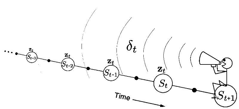
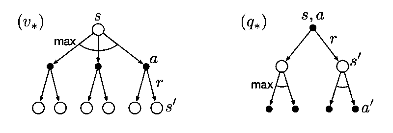Open circle represents state and solid circle represents action.

Once we have $v_*$ or $q_*$, we know optimal policy $\pi_*$ because greedy policy with respect to optimal value function is an optimal policy.

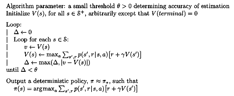
Bellman optimality equation, i.e., Bellman equation for optimal value function $v_*$ forms a system of n non-linear equations, where n is the number of states. $v_*$ can be solved if we know the dynamics which are usually unavailable. Therefore, many reinforcement learning methods can be viewed as approximately solving the Bellman optimality equation using the actual experienced transition in place of knowledge of the dynamics. Besides, computation power is also a constraint. Tasks with small state sets are possible to be solved by tabular methods ( specifically, DP). Tasks with large number of states that could hardly be entries in a table, require to build up approximations of value functions or policies.

Dynamic programming

DP uses value function to organize the search of the optimal policy given the knowledge of all components of a finite MDP. This method is limited for very large problems but it is still important theoretically for understanding other methods which attempt to achieve much the same effects but without assuming full knowledge of the environment.

Since the environment's dynamics are completely known, why not solve the system of $|S|$ linear equations with $v_\pi(s), s \in S$ as unknowns directly? Computationally expensive. Instead, DP turns Bellman equations into update rule to iteratively compute $v_\pi$.

Policy iteration

Policy iteration consists of 2 steps in each iteration:

1. Iterative policy evaluation: compute the value function $v_\pi$ for an arbitrary policy π(e.g., random policy) by repeating the following update until convergence: $$v_{k+1}(s) = \sum_a \pi(a|s) \sum_{s^\prime,r} p(s^\prime,r|s,a)[r+ \gamma v_{k}(s^\prime)]$$ One could use two arrays, one for the old values and the other for the new values. It's easier to use only one array and update the values "in place", with new values immediately overwriting old ones. This in-place algorithm converges faster. Updating estimates based on other estimates is called bootstrapping.

   Convergence proof: Bellman operator is a contraction mapping

2. Policy improvement: improve the policy by making it greedy with respect to the value of the original policy $$\pi^\prime \doteq \operatorname*{argmax}_a \sum_{s^\prime,r} p(s^\prime,r|s,a)[r+ \gamma v_\pi(s^\prime)]$$

   Why improvement is guaranteed? policy improvement theorem

The iteration loop is: $$\pi_0\xrightarrow{E}v_{\pi_0}\xrightarrow{I} \pi_1\xrightarrow{E}v_{\pi_1}\xrightarrow{I} \cdots \pi_*\xrightarrow{E}v_{\pi_*}$$ where E denotes a policy evaluation and I denotes a policy improvement.

Once a policy $\pi$ has been improved using $v_\pi$ to yield a better policy $\pi^\prime$, we can then compute $v_{\pi^\prime}$ and improve it again to yield an even better policy $\pi^{\prime\prime}$. Each policy is guaranteed to be a strict improvement over the previous one unless it is already optimal. A DP method is guaranteed to find the optimal policy in polynomial time. The algorithm is given below.

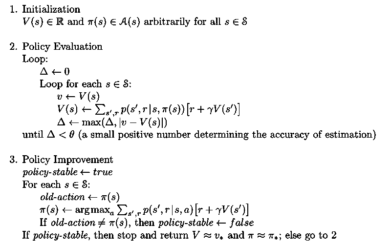
Usually, policy iteration would find the optimal policy after few iterations.

The idea of policy iteration can be abstracted as Generalized Policy Iteration (GPI) which consists of two processes: one predicts the values for the current policy and the other improves the policy wrt the current value function. They interact in such a way that they both move toward their optimal values. DP, MC and TD all follow this idea.

Value iteration

Policy evaluation requires multiple sweeps of the state set until convergence to $v_\pi$ in the limit. However, there is no need to wait until convergence before policy improvement.

Value iteration turns Bellman optimality equation into an update rule which combines one sweep of policy evaluation and policy improvement. $$v_{k+1}(s) = \max_a \sum_{s^\prime,r} p(s^\prime,r|s,a)[r+ \gamma v_{k}(s^\prime)]$$

Either policy iteration or value iteration is widely used but it is not clear which is better in general.

Monte Carlo

Only episodic tasks are considered here. Only on the completion of an episode are value estimates and policy changed. MC can learn value function based on experience (sample episodes gained through real or simulated interaction with the environment) without knowing environment dynamics. Another big difference from DP is that MC do not bootstrap (i.e., update state values on the basis of value estimates of successor states) and thus is more robust to the violence of Markov property and can evaluate a small subset of states of interest.

MC prediction (policy evaluation)

1. first visit: estimates $v_\pi(s)$ as the average return following the first visit to s in an episode
2. every visit: following every visit to s

MC control

Control problem requires to learn an action value function rather than a state value function. In this article, we often develop the ideas for state values and prediction problem, then extend to action values and control problem.

Similar to policy iteration, MC intermix policy evaluation and policy improvement steps on an episode-by-episode basis:

1. estimate action value function $q_\pi(s,a)$, the expected return when starting in state s, taking action a, and thereafter following policy $\pi$
2. improve policy by making greedy wrt $q_\pi$

Convergence to $q_\pi$ requires that all (s, a) pairs are visited an infinite number of times. In order to meet this requirement, Experience can be generated in different ways:

• exploring starts (impractical): specify an episode starts with a state-action pair and every pair has nonzero probability of being selected as the start
• on policy (soft policy): stochastic policy with a nonzero probability of selecting all actions in each state $\forall s, a \quad \pi(a|s) > 0$, e.g., ε-greedy policy. Policy iteration also works for soft policy.
• off policy: experience generated with behavior policy μ ≠ π, behavior policy μ may be uniformly random (stochastic and exploratory) while target policy π may be deterministic as long as if π(s)>0, μ(s)>0
  • of greater variance and slower to converge
  • need to apply importance sampling to estimate the expected returns (values) for target policy given the returns due to the behavior policy by weighting the return according to the relative probability of their trajectory occurring under the target and behavior policy
    • ordinary importance sampling (unbiased but larger variance)
    • weighted importance sampling (preferred)

$$v_\pi(s) = \mathbb{E}[\rho_{t:T-1}G_t | S_t=s]$$ where $\rho_{t:T}$ is importance sampling ratio: $$\begin{align} \rho_{t:T-1} &\doteq \frac{\prod_{k=t}^{T-1}\pi(A_k|S_k)p(S_{k+1},R_{k+1}|S_k,A_k)}{\prod_{k=t}^{T-1}\mu(A_k|S_k)p(S_{k+1},R_{k+1}|S_k,A_k)} \\ &= \prod_{k=t}^{T-1} \frac{\pi(A_k|S_k)}{\mu(A_k|S_k)} \end{align}$$ Let $\tau(s)$ denote the set of all time steps in which state s is visited. $v_\pi$ is estimated as: $$v_\pi(s) = \eta^{-1} \sum_{t \in \tau(s)} \rho_{t:T(t)-1} G_t$$ where $\eta = |\tau(s)|$ for ordinary whereas $\eta = \sum_{t \in \tau(s)} \rho_{t:T(t)-1}$ for weighted case.

An episode by episode incremental algorithm for MC off policy control using weighted importance sampling is shown below

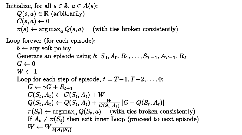
It's worth noting that ratio defined for $q_\pi$ is starting from t+1: $$\rho_{t:T-1} = \prod_{k=\boldsymbol{t+1}}^{T-1} \frac{\pi(A_k|S_k)}{\mu(A_k|S_k)}$$

Difference between on-policy and off-policy? Which is preferred?

• On-policy: estimate the value function of the policy being followed and improve the current policy
  • in order to maintain sufficient exploration (ε does not reduce to 0), it learns a near optimal policy that still explores. e.g., Sarsa learns a conservative policy in the cliff-walking task.
• Off-policy: learn the value function of the target policy from data generated by a different behavior policy
  • learn the optimal policy but the online performance of the behavior policy might be worse

Temporal-Difference learning

Like MC, TD methods use experience to evaluate policy.

Like DP, TD methods bootstrap.

TD combines the sampling of MC with bootstrapping of DP.

TD(0) prediction

TD(0) or one-step TD makes the update by $$V(S_t) \gets V(S_t) + \alpha [R_{t+1} + \gamma V(S_{t+1})- V(S_t)]$$

$R_{t+1} + \gamma V(S_{t+1})$ is update target.

$R_{t+1} + \gamma V(S_{t+1}) - V(S_t)$is called TD error.

Advantages:

• Over DP: don't require to know dynamics
• Over MC: TD target looks one time-step ahead instead of waiting until the end of an episode (online, incremental, bootstrap) and usually converge faster

TD(0) control

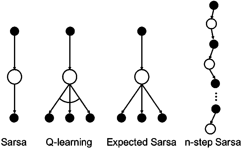
Sarsa (On-policy)

After each transition ($S_t, A_t \to R_{t+1}, S_{t+1}$), apply the following update rule: $$Q(S_t, A_t) \gets Q(S_t, A_t) + \alpha [R_{t+t}+\gamma Q(S_{t+1}, A_{t+1}) - Q(S_t, A_t)]$$ where $Q(S_{t+1}, A_{t+1}) = 0$ if $S_{t+1}$ is terminal.

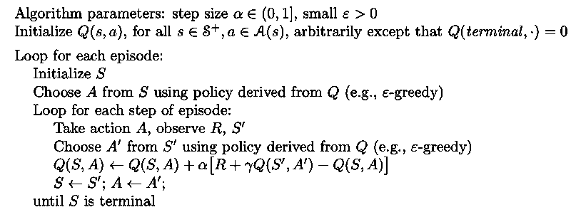
Sarsa converges to an optimal policy as long as all state-action pairs are visited infinite number of times and standard $\alpha$ reduction is meet and ε decreases to 0 in the limit.

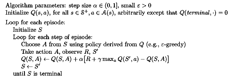
Q-learning (Off-policy)

Compared with Sarsa, the only change is the update target. $$Q(S_t, A_t) \gets Q(S_t, A_t) + \alpha [R_{t+1}+\max_a \gamma Q(S_{t+1}, a) - Q(S_t, A_t)]$$ Why is Q-learning off-policy? the policy learned is independent of the policy being followed

Why is there no importance sampling ratio?

convergence condition (minimum among all algorithms): all pairs continue to be updated plus the usual stochastic approximation conditions on the sequence of step-size parameter

Expected Sarsa

Compared with Q-learning, expected Sarsa uses expected over next state-actions pairs instead of maximum, taking into account how likely each action is under the current policy.

$$Q(S_t, A_t) \gets Q(S_t, A_t) + \alpha [R_{t+t}+ \gamma \sum_a \pi(a|S_{t+1}) Q(S_{t+1}, a) - Q(S_t, A_t)]$$

• more complex computationally but perform better than Saras and Q learning
• can use off-policy or on-policy: Q-learning is special case of off-policy when π is greedy and μ explores

Comparison of Sarsa, Q-learning and Expected Sarsa

Sarsa, Q-learning and Expected Sarsa, which is the best? Why?

No straightforward answer. It depends on the task. Despite this, here are some general conclusions:

• Sarsa: As a baseline
• Q-learning
  • pros: can learn optimal policy independent of the policy being followed while Sarsa has to gradually decrease ε to 0 to find the optimal policy; usually learns/converges faster because of the max operator in the update
  • cons: overestimation; off-policy approximation leads to divergence
• Expected Sarsa
  • pros: speed up learning by reducing variance in update; perform better at a large range of α values
  • cons: more complex computationally

Expected Sarsa generalizes Q-learning while reliably improving over Sarsa.

n-step TD

n-step TD generalizes MC and TD(0). MC performs an update for each state based on the entire sequence of rewards from that state until the end of the episode. The update of one-step TD methods, on the other hands, is based on the next reward plus the value of the state one step later. n-step TD methods use n step return as update target.

n-step on/off-policy Sarsa

$$\begin{align} G_{t:t+n} &\doteq \sum_{k=1}^n \gamma^{k-1}R_{t+k} + \gamma^n Q_{t+n-1}(S_{t+n}, A_{t+n}) \\ Q_{t+n}(S_t, A_t) & \doteq Q_{t+n-1}(S_t, A_t) + \alpha \rho_{t+1:t+n} [G_{t:t+n}-Q_{t+n-1}(S_t, A_t)] \end{align}$$ If $t+n \ge T$, all missing terms are 0, thus $G_{t:t+n}=G_t$.

Also, if two policies are the same (on-policy) then the importance sampling ratio $\rho_{t+1:t+n}$ is always 1.

Note that the ratio starts from t+1 because we are evaluating $(S_t, A_t)$ and ratio is only needed to adjust return for subsequent actions and rewards.

Drawback of n-step TD: the value function is updated n steps later, which requires more memory to record states, actions and rewards.

Planning and Learning

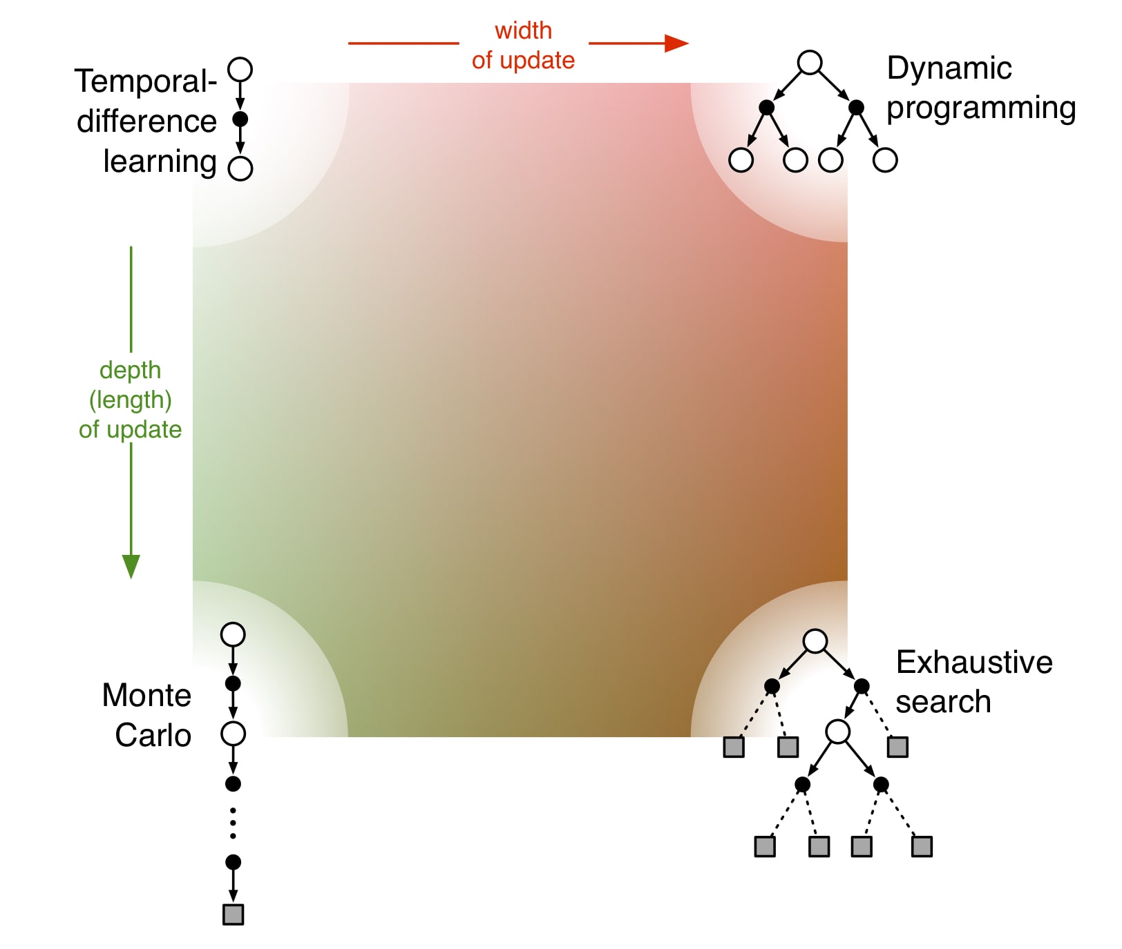
• model-based methods such as DP rely on planning
• model-free such as MC and TD rely on learning

Both planning and learning estimate value function. The difference is that planning uses simulated experience generated by a model whereas learning uses real experience generated by the environment.

There are 2 kinds of models: distribution model, such as dynamics used in DP, describes all possibilities and their probabilities while sample model produces just one possibility sampled according to the probabilities. Given a state and an action, a sample model produces a possible transition, and a distribution model generates all possible transitions weighted by their probabilities of occurring.

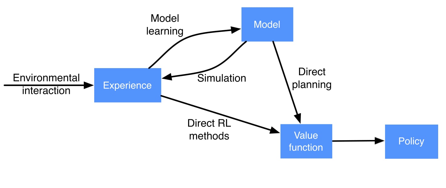
Dyna: Integrated planning, acting and learning

• planning: the model is learned from real experience and gives rise to simulated experience which backup value estimation and thus improve policy (indirect RL)
• acting: online decision making following current policy
• learning: learn value functions/policy from real experience directly (direct RL)

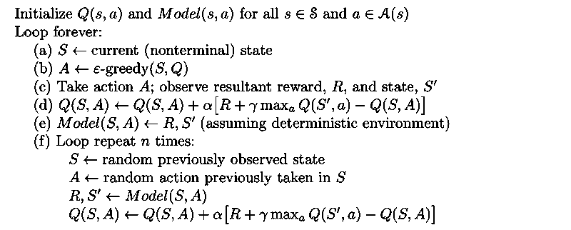
Direct reinforcement learning, model-learning, and planning are implemented by steps (d), (e), and (f), respectively.

Planning occurs in the background and samples only state-action pairs that have previously been experienced. Q-learning is used to update the same estimated value function both for learning from real experience and for planning from simulated experience.

Without (e), (f), this is exactly the Q-learning algorithm. Why planning? Planning makes full use of a limited amount of experience and thus achieve better policy with fewer environment interactions.

Improve efficiency: Prioritized sweeping helps to increase the speed to find optimal policy dramatically by working backward from states whose value has changed instead of sampling state-action pairs randomly.

Rollout: Online planning

Rollout is executed to select the agent's action $A_t$ for current state $S_t$. It aims to improve over the current policy.

1. estimate action values for current state and for rollout policy
   1. sample many trajectories starting from the current state with a sample model following rollout policy
   2. average returns of these simulated trajectories. how? the value of a state-action pair in the trajectory is estimated as the average return from that pair.
2. select an action that maximizes these estimates. This results in a better policy than the rollout policy. Rollout planning is a kind of decision-making planning because it makes immediate use of these action-value estimates at decision time, then discard them.
3. Repeat 1-2 for next state

Monte Carlo Tree Search

MCTS is a rollout algorithm but enhanced by accumulating value estimation obtained from sample trajectories. It stores partial Q as a tree rooted at the current state: each node represents a state and the edge between 2 states represents an action.

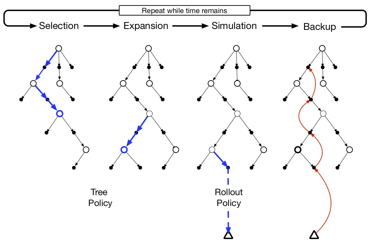
Each execution of MCTS consists the following 4 steps as shown in the figure above:

1. Selection: traverse the tree from root to a leaf node following a tree policy, such as $\epsilon$-greedy or UCB selection rule, based on action values attached to edges
2. Expansion: expand from the selected leaf node to a child node
3. Simulation: simulate a complete episode from the expanded node to a terminal state following rollout policy
4. Backup: the rewards generated by the simulated episode are used to update value of actions selected by tree policy

After repeating the above iteration until time limit reaches, an action from the root state is selected. how? maximum action value or most frequently visited. After transition to next state, a subtree starting from the new state will be used.

Value function approximation (mainly linear FA)

The approximate value function is not represented by a table but by a parameterized functional form with weight vector $\mathbf{w} \in \mathbb{R}^d$. $$\hat{v}(s,\mathbf{w}) \approx v_\pi(s)$$ Function approximation $\hat{v}(s,\mathbf{w})$ can be any supervised Machine Learning methods that learn to mimic input-output examples (output/prediction is number) such as a linear function or neural network.

• Compact: The number of parameters is much less than the number of states (infinite for continuous state space). It is impossible to get all values exactly correct.
• Generalize: changing one weight changes the estimated value of many states. If the value of a single state is updated, the change affects the values of many other states.
• Online: learn incrementally from data acquired while the agent interacts with the environment

The objective function to minimize is mean squared value error: mean squared error between the approximate value and the true value over the state space $$\overline{VE} = \sum_{s \in S} \mu(s) [\hat{v}(s,\mathbf{w}) - v_\pi(s)]^2$$

Stochastic gradient descent based methods

SGD is the most widely used optimization algorithm. The approximate value function is a differentiable function of $\mathbf{w}$ for all $s \in S$. An input-output exapmle consists of a state and its true value: $S_t \rightarrow v_\pi(S_t)$. SGD adjusts weights after each training example: $$\begin{align} \mathbf{w}_{t+1} &\doteq \mathbf{w}_t - \frac{1}{2} \alpha \nabla [v_\pi(S_t) - \hat{v}(S_t,\mathbf{w}_t)]^2 \\ &= \mathbf{w}_t + \alpha [v_\pi(S_t) - \hat{v}(S_t,\mathbf{w}_t)] \nabla \hat{v}(S_t,\mathbf{w}_t) \end{align}$$ Since $v_\pi(S_t)$ is unknow, an estimate $U_t$ will substitute it. $$\mathbf{w}_{t+1} \doteq \mathbf{w}_t + \alpha [U_t - \hat{v}(S_t,\mathbf{w}_t)] \nabla \hat{v}(S_t,\mathbf{w}_t)$$ It guarantees to converge to a local optimum if α satisfies the standard stochastic approximation conditions.

• true gradient
  • MC update is an unbiased estimate of the true value $v_\pi(S_t)$ because $\mathbb{E}[G_t] = v_\pi(S_t)$
  • convergence guaranteed
• semi-gradient
  • updates which bootstrap such as DP and n-step TD targets depend on the approximate values and thus on weights. They are biased and the update rule includes only a part of the gradient.
  • converge in linear case
  • advantages:
    • learn faster
    • online without waiting for the end of an episode

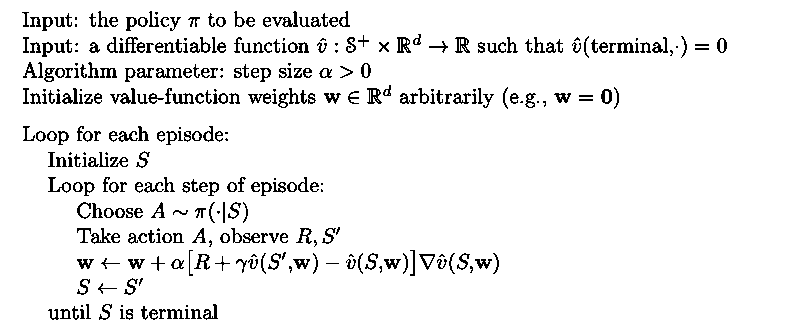
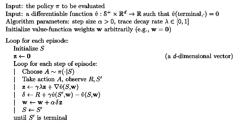
Complete algorithm for Semi-gradient TD(0) which uses $U_t \doteq R_{t+1}+\gamma \hat{v}(S_{t+1}, \mathbf{w})$ as its target is as below:

Linear function approximation

The approximation function is saied to be linear if the approximate state-value function is the inner product between the state (a real-valued feature vector $\mathbf{x}(s) = (x_1(s), x_2(s),\cdots, x_d(s))^\top$) and weight vector $\mathbf{w}$. $$\hat{v}(s) \doteq \mathbf{w}^\top \mathbf{x}(s) \doteq \sum_{i=1}^d w_i x_i(s)$$

Combined with SGD, the gradient of linear function wrt $\mathbf{w}$ is $\mathbf{x}(s)$. Thus, the SGD update becomes: $$\mathbf{w}_{t+1} \doteq \mathbf{w}_t + \alpha [U_t - \hat{v}(S_t,\mathbf{w}_t)] \mathbf{x}(S_t)$$

In this case, true gradient methods converge to global optimum while semi-gradient methods converge to a TD fixed point (a point near local optimum).

State representation (feature engineering) for Linear approximation

• state aggregation: reduce the number of states by grouping nearby states as a super state which has a single value

Linear methods cannot take into account the interaction between different features in the natural state representation. Therefore, additional features are needed. Subsequent ways are all dealing with this problem.

• polynomials: e.g., expand $(x_1,x_2)$ to $(1,x_1,x_2,x_1x_2)$
• coarse coding: in a 2D continuous state space, a state/point is encoded as a binary vector each value/feature corresponding to a circle in the space. 1 means the point is present in the circle and 0 means absence. Circles can be overlapping. Size, density (number of features) and shape of receptive fields (e.g., circles) have effect on the generalization.
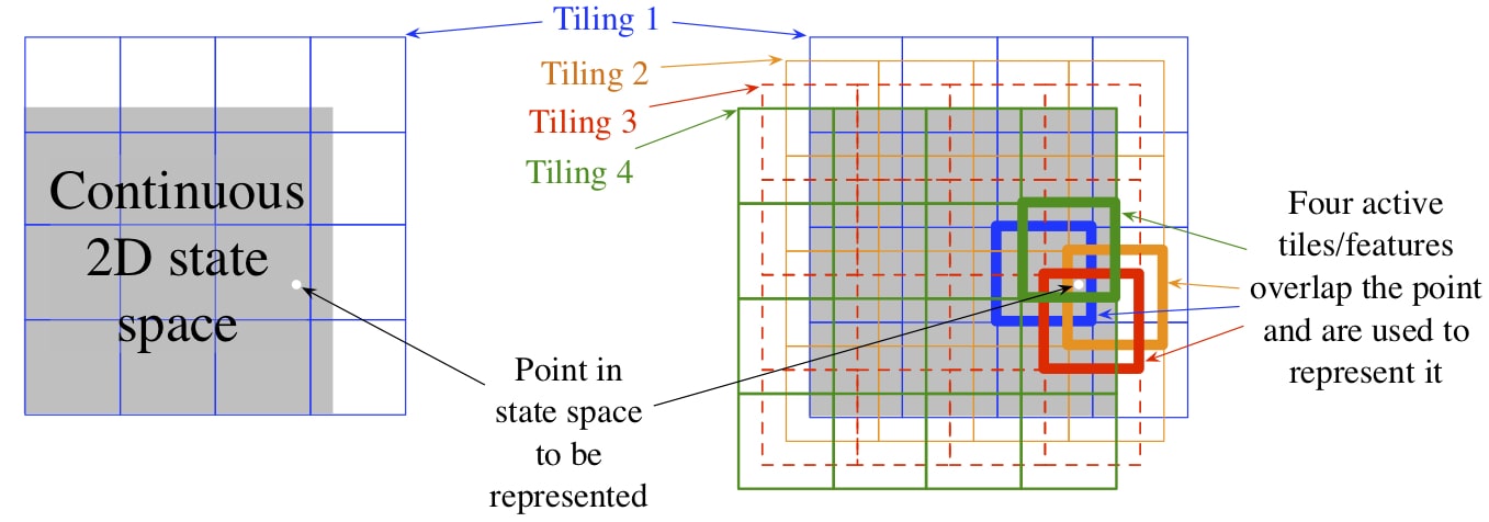
• tile coding: a form of coarse coding more flexible and computationally efficient for multi-dimensional space:
  • efficient: in linear FA, the weighted sum involves d multiplications and additions. Using tile coding, specifically, binary feature vector, one simply computes the indices of n << d active features and add up the n relevant weights
  • flexible: number, shape of tiles and offset of tilings can affect generalization
    • number of tilings (or features) determines the fineness of the asymptotic approximation
    • shape: use different shaped tiles (vertical, horizontal, conjunctive rectangle tiles) in different tilings
    • offset: uniform offset results in strong effect along the diagonal and asymmetric offset may be better
• Radial Basis Function: greater computational complexity and more manual tuning
• Fourier Basis: performs better than polynomials and RBF

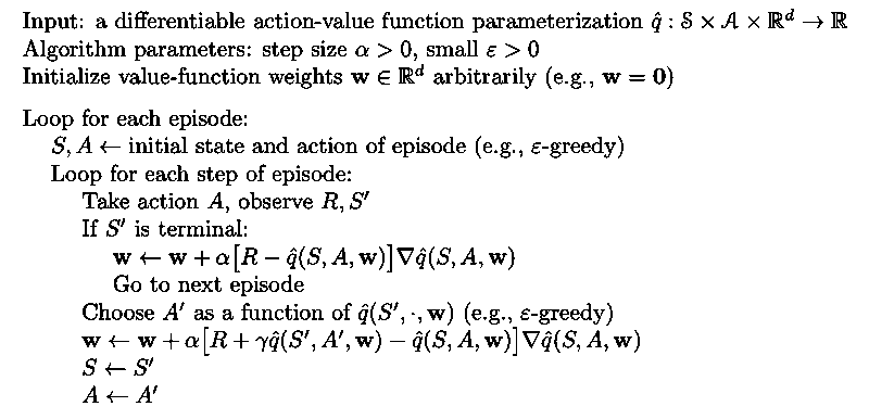
On-policy control: Episodic Semi-gradient Sarsa

Let's consider control problem, SGD update for action-value is $$\mathbf{w}_{t+1} \doteq \mathbf{w}_t + \alpha [U_t - \hat{q}(S_t,A_t,\mathbf{w}_t)] \nabla \hat{q}(S_t,A_t,\mathbf{w}_t)$$

For one-step Sarsa, $$\mathbf{w}_{t+1} \doteq \mathbf{w}_t + \alpha [R_{t+1} + \gamma \hat{q}(S_{t+1}, A_{t+1}, \mathbf{w}) - \hat{q}(S_t,A_t,\mathbf{w}_t)] \nabla \hat{q}(S_t,A_t,\mathbf{w}_t)$$

Episodic on-policy one-step semi-gradient Sarsa is shown below:

Off-policy control

Function approximation methods with off-policy training do not converge as robustly as they do under on-policy training. Off-policy can lead to divergence if all of the following three elements are combined (deadly triad):

1. function approximation: scale to large problem
2. bootstrapping: faster learning
3. off-policy: flexible for balancing exploration and exploitation

Importance sampling for off-policy tabular methods attempts to correct the update targets but still doesn't prevent from divergence in function approximation cases. The problem of off-policy learning with function approximation is that the distribution of updates doesn't match the on-policy distribution. There are 2 possible fixes:

1. use importance sampling to warp update distribution back to the on-policy distribution
2. develop true gradient methods that do not rely on special distribution for stability

Eligibility traces

When n-step TD methods are augmented by eligibility traces, they learn more efficiently:

1. no delay: learning occurs continually in time rather than being delayed n steps
2. only store a single trace vector (short-term memory)

We will focus on function approximation although it also works for tabular methods.

λ-return and forward-view

n-step return or update target is: $$G_{t:t+n} = R_{t+1} + \cdots + \gamma^{n-1}R_{t+n} + \gamma^n \hat{v}(S_{t+n}, \mathbf{w}_{t+n-1})$$

Compound update is average of n-step returns for different ns. e.g., half of a two-step return and half of a four-step return is $\frac{1}{2} G_{t:t+2} + \frac{1}{2} G_{t:t+4}$

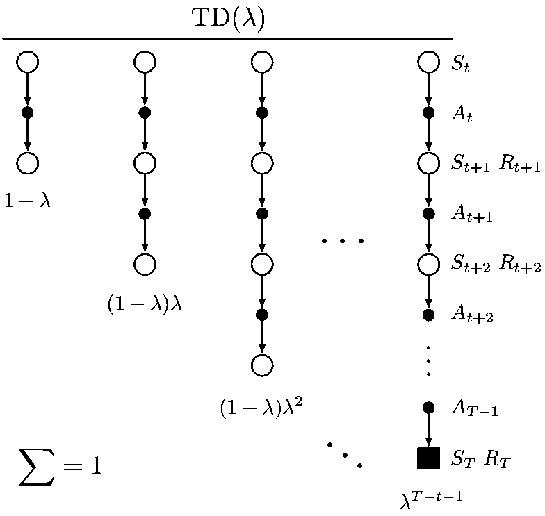
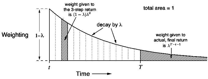
λ-return is one particular way of averaging n-step returns $$\begin{align} G_t^\lambda &= (1-\lambda) \sum_{n=1}^\infty \lambda^{n-1}G_{t:t+n} \\ &= (1-\lambda) \sum_{n=1}^{T-t-1} \lambda^{n-1}G_{t:t+n} + \lambda^{T-t-1}G_t \end{align}$$ where decay factor $\lambda \in [0,1]$:

• λ=1, λ-return is $G_t$, the MC target
• λ=0, λ-return reduces to $G_{t:t+1}$, the one-step target

That's why eligibility traces can also unify and generalize MC and TD(0) methods.

The backup diagram and the weighting on the sequence of n-step returns in the λ-return are shown below:

offline λ-return algorithm

At the end of an episode, a whole sequence of offline updates are made according to the Semi-gradient rule, using λ-return as the target: $$\mathbf{w}_{t+1} \doteq \mathbf{w}_t + \alpha \left[G_t^\lambda-\hat{v}(S_t,\mathbf{w}_t)\right] \nabla\hat{v}(S_t,\mathbf{w}_t), t=0,1,\cdots, T-1$$

truncated λ-return algorithm

λ-return is unknown until the end of episode. longer-delayed rewards are weaker because of the decay $\lambda$ for each step. They can be replaced with estimated value.

truncated λ-return is: $$G_{t:h}^\lambda = (1-\lambda) \sum_{n=1}^{h-t-1} \lambda^{n-1}G_{t:t+n} + \lambda^{h-t-1}G_{t:h}$$ truncated TD(λ): truncated λ-return algorithm in state value case $$\mathbf{w}_{t+n} \doteq \mathbf{w}_{t+n-1} + \alpha \left[G_{t:t+n}^\lambda-\hat{v}(S_t,\mathbf{w}_{t+n-1})\right] \nabla\hat{v}((S_t,\mathbf{w}_{t+n-1}), \quad 0 \le t < T$$

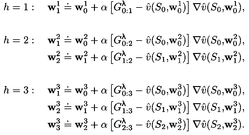
Online λ-return algorithm: Perform better (currently the best performing TD method but computationally expensive) by redoing updates since beginning of episode at each time step. $$\mathbf{w}_{t+1}^h \doteq \mathbf{w}_t^h + \alpha \left[G_{t:h}^\lambda-\hat{v}(S_t,\mathbf{w}_t^h)\right] \nabla\hat{v}(S_t,\mathbf{w}_t^h), 0 \le t < h \le T$$

The first three update sequences are shown below:

backward-view

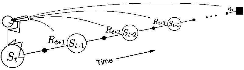
• forward-view: the value update is based on future states and rewards. Simple for theory and intuition.
• backward-view: look at the current TD error and assign it backward to prior states. Backward-view algorithm is a more efficient implementation form of forward-view algorithm using eligibility traces.

The difference between forward-view and backward-view is illustrated below:

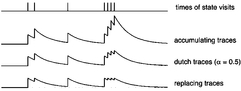
eligibility traces: $$\mathbf{z}_{-1} = \mathbf{0} \\ \mathbf{z}_t = \lambda\gamma\mathbf{z}_{t-1} + \nabla v(S_t, \mathbf{w}_t), 0 \le t \le T$$ This vector indicates the eligibility for change of each component of the weight vector.

This is accumulating traces, there are also Dutch and replacing traces. Their difference is illustrated below:

Semi-gradient version of TD(λ) with function approximation

TD(λ) improves over offline λ-return algorithm by looking backward and updating at each step (online). Ironically, TD(λ) doesn't use one-step return instead of λ-return. $$\delta_t \doteq R_{t+1} + \gamma \hat{v}(S_{t+1},\mathbf{w}_t) - \hat{v}(S_t,\mathbf{w}_t) \\ \mathbf{w}_{t+1} \doteq \mathbf{w}_t + \alpha \delta_t \mathbf{z}_t$$

where $\delta_t$ is one step TD error.

TD(1) is a more general implementation of MC algorithm:

1. continuing, not limited to episodic tasks
2. online, policy is improved immediately to influence following behavior instead of waiting until the end

True online TD(λ)

TD(λ) algorithm only approximates online λ-return algorithm. True online TD(λ) inverts the forward-view online λ-return algorithm for the case of linear FA to an efficient backward-view algorithm using eligibility traces.

The sequence of weight vectors produced by online λ-return algorithm is:

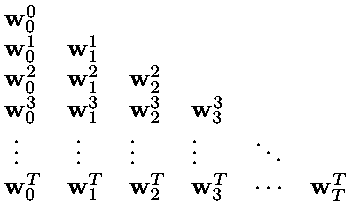
True online TD(λ) computes just the sequence of $w_t^t$ by $$\mathbf{w}_{t+1} \doteq \mathbf{w}_t + \alpha \delta_t \mathbf{z}_t + \alpha(\mathbf{w}_t^\top\mathbf{x}_t - \mathbf{w}_{t-1}^\top\mathbf{x}_t)(\mathbf{z}_t-\mathbf{x}_t)$$ where $z_t$ is Dutch trace: $$\mathbf{z}_t \doteq \gamma\lambda \mathbf{z}_{t-1} + (1-\alpha\gamma\lambda \mathbf{z}_{t-1}^\top \mathbf{x}_t)\mathbf{x}_t$$

This algorithm produces the same sequence of weight vectors as the online λ-return algorithm but less expensive (complexity is the same as TD(λ))

Control with Eligibility traces: Sarsa(λ)

Sarsa(λ) is the control/action-value version of TD(λ) with state-value function being replaced by action-value function. $$\mathbf{w}_{t+1} \doteq \mathbf{w}_t + \alpha \delta_t \mathbf{z}_t \\ \delta_t \doteq R_{t+1} + \gamma \hat{q}(S_{t+1},A_{t+1},\mathbf{w}_t) - \hat{q}(S_t,A_t,\mathbf{w}_t) \\ \mathbf{z}_{-1} = \mathbf{0}, \mathbf{z}_t = \lambda\gamma\mathbf{z}_{t-1} + \nabla q(S_t, A_t, \mathbf{w}_t), 0 \le t \le T$$

The fading-trace bootstrapping strategy of Sarsa(λ) increases the learning efficiency, which is shown in the gridworld example below. All rewards were zero except a positive reward at the goal location.

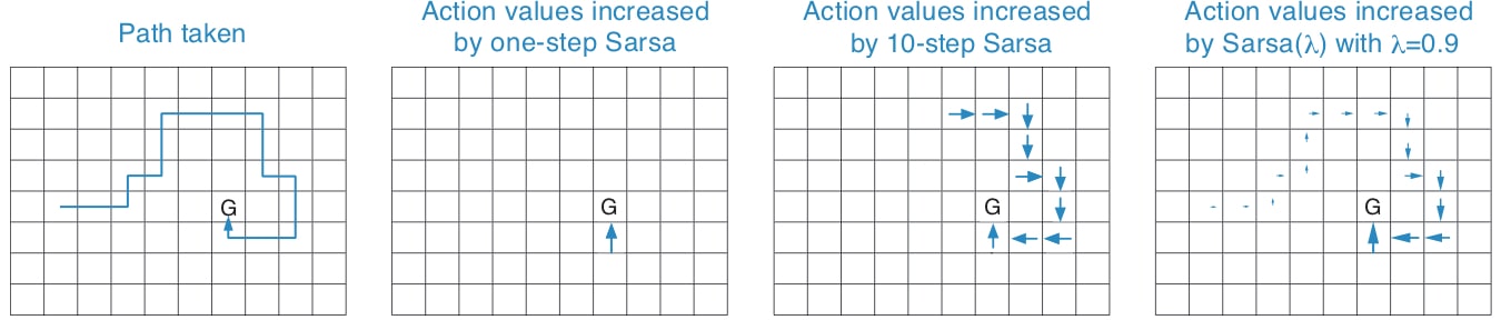
One-step would increment only the last action value, whereas n-step method would equally increment the last n actions' values, and an eligibility trace method would update all the action values up to the beginning of the episode, to different degrees, fading with recency.

Similarly, true online Sarsa(λ) is the action-value version of True online TD(λ). True online Sarsa(λ) performs better than regular Sarsa(λ).

Comparison of MC, TD(0), TD(n), TD(λ)

Both TD(n)and TD(λ) generalize MC and TD(0).

• MC
  • Pros
    • don't bootstrap
      • have advantages in partially non-Markov tasks
      • can focus on a small subset of states
    • model-free (over DP): learn optimal policy directly from interaction with the environment or sample episodes, with no model of the dynamics which is required by DP
  • Cons
    • update delayed until the termination, not applicable for continuing task
    • high variance and slow convergence
• TD(0)
  • Pros
    • fast because of (over MC) update at each step without delay and (over other) simple equation with minimum amount of computation: suitable for offline application in which data can be generated cheaply from an inexpensive simulation and the objective is simply to process as much data as possible as quickly as possible
• TD(n)
  • Pros
    • typically performs better (faster) at an intermediate n than either extreme (i.e., TD(0) and MC) because it allows bootstrapping over multiple time steps
    • conceptually simple/clear (over TD(λ))
  • Cons (compared with TD(0))
    • update delayed n time steps
    • require more memory to record states, actions and rewards
• TD(λ)
  • Pros
    • faster learning particularly when rewards are delayed by many steps because the update is made for every action value in the episode up to the beginning, to different degrees. It makes sense to use TD(λ) in online application where data is scarce and cannot be repeatedly processed
    • efficient (over n-step method): only need to store a trace vector
  • Cons
    • require more computation (over one-step method)

Policy Approximation

Previously, policy was generated implicitly (e.g., ε-greedy) from value function approximated by parameterized function.

Now, policy approximation learns a parameterized policy that can select actions without consulting a value function. Actually, value function may still be used to learn the policy parameters but is not required to select actions. Methods that learn approximation to both policy and value function are called actor-critic methods, where actor refers to the learned policy and critic refers to the learned value function.

Advantages of policy approximation include:

1. can learn stochastic policy that enables to select actions with arbitrary probabilities
2. efficient in high dimensional or even continuous action space
3. inject prior knowledge to the policy directly
4. stronger convergence guarantees

Policy Gradient

The goal is to learn a policy $$\pi(a|s, \theta) = Pr\{A_t=a|S_t=s,\theta_t = \theta\}$$ which decides the probability of selecting action a in state s with parameter weight θ at each time step.

How to find the optimal parameter θ?

We only consider a family of methods called policy gradient methods which maximize a scalar performance $J(\theta)$ using gradient ascent. $$\theta_{t+1} = \theta_t + \alpha \nabla J(\theta_t)$$ where column vector $\nabla J(\theta)$ is the gradient of the performance measure wrt components of its arguments θ: $$\nabla J(\theta) = (\frac{\partial{J(\theta)}}{\partial{\theta_1}}, \cdots, \frac{\partial{J(\theta)}}{\partial{\theta_d}})$$ This requires the policy function to be differentiable wrt the parameter.

How to parameterize policy?

• discrete action space: softmax $$\pi(a|s, \theta) \doteq \frac{e^{h(s,a,\theta)}}{\sum_b e_{h(s,b,\theta)}}$$ action preference h can be parameterized by linear function or neural network

• continuous action space: normal/Gaussian distribution $$\pi(a|s,\theta) = \frac{1}{\sigma(s,\theta)\sqrt{2\pi}} exp(-\frac{(a-\mu(s,\theta))^2}{2\sigma(s,\theta)^2})$$ The policy is determined by the mean μ and standard deviation σ which are parameterized functions that depend on state s.

What is the performance measure or objective function?

• episodic tasks: the measure is the value of the start state of the episode, i.e., the return of the whole episode $$J(\theta) \doteq v_{\pi_\theta}(S_0)$$

• continuing tasks: use average reward: $$J(\theta) \doteq \sum_s P_\pi(s) \sum_a \pi(a|s,\theta) \sum_{s^\prime,r} p(s^\prime, r|s,a) r$$ where $P_\pi(s)$ is steady state distribution under π.

With policy gradient, we need to improve the policy performance by adjusting the policy parameter using the gradient of performance wrt policy parameter.

How to compute the gradient of performance wrt policy parameter?

The return of an episode depends on which actions are selected and which states are encountered. The effect of the policy parameter on action selection, and thus on return, can be computed in a straightforward way from the parameterized policy function. But it is not possible to compute the effect of the policy parameter on state distribution because state distribution depends on environment dynamics which are typically unknown.

The policy gradient theorem solves this problem (doesn't require the derivative of dynamics) and establishes: $$\nabla J(\theta) = \sum_s d_\pi(s) \sum_a q_\pi(s,a) \nabla \pi(a|s, \theta)$$ where $d_\pi(s)$ is the state distribution under policy π.

This theorem provides theoretical foundation for all policy gradient methods below.

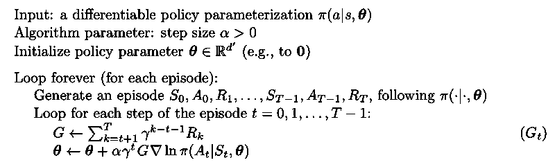
REINFORCE: Monte Carlo Policy Gradient

REINFORCE derives the policy gradient theorem by replacing the gradient with samples such that the expectation of the sample gradient is propotional to the actual gradient $$\begin{align} \nabla J(\theta) &= \sum_s d_\pi(s) \sum_a q_\pi(s,a) \nabla \pi(a|s, \theta) \\ &= \mathbb{E_\pi}\left[\sum_a q_\pi(S_t,a) \nabla \pi(a|S_t, \theta)\right] \\ &= \mathbb{E_\pi}\left[\sum_a \pi(a|S_t, \theta) q_\pi(S_t,a) \frac{\nabla \pi(a|S_t, \theta)}{\pi(a|S_t, \theta)}\right] \\ &= \mathbb{E_\pi}\left[q_\pi(S_t,A_t) \frac{\nabla \pi(A_t|S_t, \theta)}{\pi(A_t|S_t, \theta)}\right] \\ &= \mathbb{E_\pi}\left[q_\pi(S_t,A_t) \nabla \ln{\pi(A_t|S_t, \theta)} \right] \\ &= \mathbb{E_\pi}\left[ G_t \nabla \ln{\pi(A_t|S_t, \theta)} \right] \end{align}$$ and then yields the REINFORCE update: $$\theta_{t+1} = \theta_t + \alpha G_t \nabla \ln{\pi(A_t|S_t, \theta_t)}$$

The update will favor actions that yield high return.

$G_t$ is the return from time t up until the end of the episode. All updates are made after the episode is completed.

This algorithm converge to a local optimum under the standard α condition

Like all MC methods:

• high variance
• slow learning
• has to wait until end of episode, inconvenient for online or continuing problem

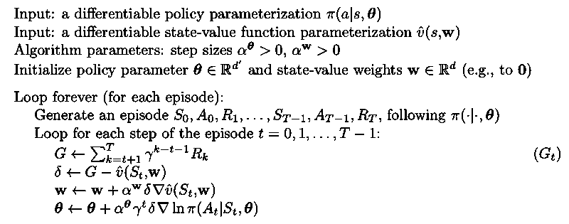
REINFORCE with Baseline

Introduce a baseline to the update of REINFORCE. $$\theta_{t+1} = \theta_t + \alpha(G_t - b(S_t)) \nabla \ln{\pi(A_t|S_t, \theta)}$$ The baseline $b(S_t)$ doesn't change the expectation but can significantly reduce variance in updates and thus speedup learning. Actually, the baseline is a state value function. If all actions in a state have high values, a baseline should have high value for that state. The action value is compared with the baseline to distinguish higher valued actions from the less highly valued ones.

Algorithm for REINFORCE with baseline using a learned state value function as the baseline is given below:

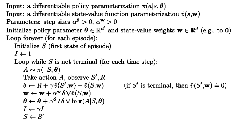
Actor-Critic Methods

To gain the advantages of TD methods, One-step actor–critic methods replace the full return in REINFORCE with one-step return and also use a learned state value function as baseline and also for bootstrapping as follows: $$\theta_{t+1} = \theta_t + \alpha(R_t+\gamma \hat{v}(S_{t+1}, \mathbf{w}) - \hat{v}(S_t, \mathbf{w})) \nabla \ln{\pi(A_t|S_t, \theta)}$$

Algorithm of Semi-gradient TD(0) with PG is shown below:

The implementation of the REINFORCE and one-step Actor-Critic as well as some more advanced deep RL methods such as DQN in Pytorch can be found here.