Overview of NLP

In this article, I will introduce many basic tasks in NLP and then present linguistic concepts and computational methods to solve them.

Morphology and Finite State Machines

Tasks

• Given a wordform, recognize if it is in a specific language
• Given the lemma and morphological properties, inflect the correct wordform
• Given a wordform, analyze the lemma and morphological properties

Morphology

Morphology is the study of word formation. Wordform signals difference in meaning.

• Stem: part of a word that is common in all its variants (e.g. stem of produce, production is produc)
• Lemma: the dictionary form of a word (e.g. lemma of fly, flies, flew and flying is fly)

• Affixes: suffix, prefix (e.g. +ed, un+)

• Inflectional morphology: use suffix to express grammatical features or syntactic relations

  • nouns for count (+s) and possessive case (+'s)
  • verbs for tense (+ed, +ing) and 3rd single person (+s)
  • adj in comparative (+er) and superlative forms (+est)
• Derivational morphology: change the part of speech or meaning of a word to create a new word e.g. word->wordify

Finite State Machine (FSM)

A word can be generated by moving from the start state to end state, emitting symbol/letter on each transition. Equivalently, a word can be recognized by matching input characters to emission letters.

FSM define a set of words or a formal/regular language. It can represent infinite language.

Why not use a mapping from a lemma to all its morphological forms?

1. too long
2. fail for productive language because such language is infinite

How is FSM used for morphological recognition, generation and analysis?

Constructing a single FSM is very complicated. This could be solved by building separate FSMs for lexicon of lemmas, inflectional and derivational morphology and then concat them. A FSM is used to recognize wordforms and a Finite State Transducer (FST) is needed to recognize morphological properties or generate surface form.

For example, walk+V+past -> walked can be generated by the FST below.

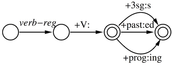
When accounting for spelling changes, the first FST generates an intermediate form and the second FST generates the surface form. E.g. bake+V+past -> bake^ed# -> baked.

Another related task: minimum edit distance

Given 2 wordforms, how "similar" are they in terms of spelling?

This similarity could indicate morphological relationship: walk - walks. The solution is minimum edit distance which measures the minimum modification needed to change word1 to word2 or vice versa.

Let ins/del cost (i.e. distance) = 1 and sub cost = 2. The minimum distance or best alignment between STALL and TABLE is D(STALL, TABLE) = 4.

STALL
 TALL  deletion
 TABL  substitution
 TABLE insertion

D(w1[:i], w2[:j]) = 
MIN(
    D(w1[:i-1], w2[:j]) + 1
    D(w1[:i], w2[:j-1]) + 1
    D(w1[:i-1], w2[:j-1]) + 2 or 0
)

Language modelling using N-grams

A Language model can tell us how likely a sentence or a sequence of words is to occur in natural language (i.e. the probability of a sentence). It's important to decide between similar sounding options (word choices) in automatic speech recognition and decide the word choices and ordering in machine translation to generate best-guess output.

Probability estimation example

1. weather forecast: What's the probability that it will rain tomorrow? To answer this question, we need data and model.

   • data: relevant information about the observed data; historic data and outcome to train the model
   • model: equations to estimate the probability

2. coin estimation:[TBD: example] fair and unfair coin models show different models will yield different estimate with the same observed data. A generative model is the probabilistic process that describes how the data is generated. A model is defined by its equations and parameters which are determined using the training data.

3. height of females: Assume the heights follow a normal distribution with parameters $(\mu, \sigma)$ or a mixture model of 2 Gaussians with 5 parameters. Incorrect model that doesn't match the data distribution will produce inaccurate result.

4. M&M colors: P(red) is estimated by relative frequency which converges to the true probability as the number of observations approaches infinity.

Relative frequency estimation in example 4 is also called Maximum likelihood estimation (MLE).

Noisy channel framework

Noisy channel framework is used to determine the best guess in the previous mentioned tasks, namely, speech recognition, machine translation and spelling correction. Given some observation x (input), we want to recover the most probable y (ouput) that is intended. The noise channel framework can be written using bayes rule: $$\underset{y}{\mathrm{argmax}} P(y|x) = \underset{y}{\mathrm{argmax}} \frac{P(x|y)P(y)}{P(x)} = \underset{y}{\mathrm{argmax}} P(x|y)P(y)$$ P(Y) is a language model. P(X|Y) is a noise model which is trained on input/output pairs.

Take the spelling correction as an example,

• X is typed words
• Y is true words
• P(Y) is the distribution over the words a user intended to type
• P(X|Y) is the distribution over what a user is likely to type, given what they meant

N-gram

How do we build a language model? It won't work by directly estimating the probability of each full sentence using MLE due to sparse data problem.

N-gram is a kind of language model.

Take bigram as an example,

$$\begin{align} P(\vec{w}) &= P(w_1 \cdots w_n) \\ &= P(w_n|w_1 \cdots w_{n-1}) P(w_{n-1}|w_1 \cdots w_{n-2}) \cdots P(w_1) \\ &\approx P(w_n|w_{n-1})P(w_{n-1}|w_{n-2}) \cdots P(w_1) \end{align}$$

• step 1: rewrite using chain rule
• step 2: make an independence assumption. According to Markov assumption: only a finite history matters, bigram assumes only one word history.

Finally,

$$\begin{align} P(\vec{w}) = \prod_{i=1}^{n+1} P(w_i|w_{i-1}) \end{align}$$

where $w_0$ = <s> and $w_{n+1}$ = </s> are used to capture behavior at the beginning and end of a sentence and $P(w_0) = 1$.

Probabilities of bigrams are estimated using MLE $P(w_2|w_1) = \frac{C(w_1, w_2)}{C(w_1)}$ over a large text corpus.

Evaluation

How good is the language model? Perplexity

$$\begin{align} PP_M(\vec{w}) &= 2^{H_M(\vec{w})} \\ H_M(\vec{w}) &= -\frac{1}{n}\log_2 P_M(w_1 \cdots w_n) \end{align}$$

Perplexity is based on cross entropy. Cross entropy measures the difference between 2 probability distribution. It's usually used to answer: how close is the predicted distribution to the true distribution? The smaller, the closer. Here, cross entropy is computed against the uniform distribution probabilities. So, the cross entropy is actually the average negative log probability of each word. Basically, the smaller the perplexity, the better the model.

Perplexity can also be used to determine the language of a document by comparing the perplexities computed by models trained on different languages. The model which yields the smallest perplexity reveals the language of the document.

Smoothing

The problem with MLE is that it estimates probabilities that make the observed data maximally probable by assuming unseen n-grams have zero probability. Any sentence with such a n-gram will be assigned probability 0. That is, it overfits the training data.

Events that never have occurred don't necessarily have zero probabilities. Most sentences have never occurred in corpus but are meaningful and grammatical. So they should have non-zero probabilities.

Smoothing is used to avoid zero probability.

Add-α Smoothing

$$P(w_{i-1}, w_i) = \frac{C(w_{i-1}, w_i) + \alpha}{C(w_{i-1}) + \alpha v}$$ Usually, α<1. If α=1, it's add-one smoothing. It reassign too much from observed to non-observed n-grams. It's common to use training/dev/test split to optimize the parameter α. Development/validation set is used to evaluate different models and optimize the parameters. Test set is used once the model and parameters are chosen.

Interpolation and backoff

Add-α assigns equal probability to all unseen n-grams. It might be better to use information from lower order (shorter n-grams).

• high-order N-grams: sensitive to context but have sparse counts
• low-order N-grams: consider only limit context but have robust counts

There are 2 ways to combine high-order and low-order N-grams.

interpolation

$$P(w_3|w_1, w_2) = \lambda_1 P(w_3) + \lambda_2 P(w_3|w_2) + \lambda_3 P(w_3|w_1, w_2)$$ $\lambda_i$s are interpolation parameters which can be fitted on a training set and chosen to optimize perplexity on a held-out set.

back-off

Basic idea: Trust a high-order model if it contains the N-gram otherwise "back off" to a lower order model. In the previous example, if the trigram has zero probability, it will use the probability of the bigram. Maths get complicated because the probability given a history has to sum up to 1.

Kneser-Ney smoothing

The previous methods still have problems. For example, the word York is very common but it always directly follows New. The unigram model has a respectable high probability. In unseen N-gram context, P(York|w) should have low probability. However, the interpolation or back-off uses probability predicted by unigram model which is high.

Kneser-Ney takes diversity of history into account. It replaces raw count by distinct count of one word history in unigram language model.

$$C^\prime(w_i) = |\\{w_{i-1}: C(w_{i-1}, w_i)>0\\}| \\ P(w_i) = \frac{C^\prime(w_i)}{\sum_{w_j}{C^\prime(w_j)}}$$

Text categorization using Naive Bayes classifier

Text categorization is a classification task. Some examples:

1. spam detection
2. sentiment analysis
3. topic classification
4. authorship attribution
   1. native language identification
   2. diagnosis of disease
   3. identification of gender, dialect, educational background

Bag-of-words model

Given document d with features $f_1, f_2, \dots,f_n$ and set of categories C. The formula of Naive Bayes classifier is:

$$\begin{align} \hat{c} = \underset{c \in C}{argmax}P(c|d) = \underset{c \in C}{argmax} \frac{P(d|c)P(c)}{P(d)} = \underset{c \in C}{argmax} P(d|c)P(c) \end{align}$$

document representation

• each document is represented by a bag of words
• usually use binary feature values (whether a unigram/word occurs in a document or not)
• usually exclude stopwords or only choose a small task relevant set (e.g. sentiment lexicon)
• need independence assumption

$$\begin{equation} \hat{c} \approx \underset{c \in C}{argmax} P(c) \prod_{i=1}^{n} P(f_i|c) \end{equation}$$

class priors are estimated with MLE

$$\begin{equation} \hat{P}(c) = \frac{N_c}{N} \end{equation}$$

feature probabilities are estimated using counts with α smoothing (TBD: is it correct to use frequency in this model?)

$$\begin{equation} \hat{P}(f_i|c) = \frac{count(f_i, c) + \alpha}{\sum_{f \in F}{(count(f, c) + \alpha)}} \end{equation}$$

Pros and Cons

• pros: simple to implement and fast to train
• cons: rely on strong assumption. Features are usually not independent given the class and the decision will be overconfident.

Evaluation

• intrinsic: measures inherent to the task (accuracy, F-score)
  • For unbalanced classes, tune the threshold on posterior probability to get desired precision or recall. For example, system returns Y when $P(Y|d) > t$.
  • F measure penalizes large difference between P and R.
• extrinsic: measure effects of a downstream task

Part-of-speech tagging using Hidden Markov Model

Given a sequence of words, what's the most probable tag sequence for the sentence?

There are 2 kinds of POS tags

• open class words (content words): nouns, verbs...
• closed class words (function words): pronouns, determiners...

POS tagging is hard because

1. ambiguity: homographs
2. sparse data

Hidden Markov Model

HMM is a probabilistic model for POS tagging and other sequence labeling tasks.

HMM defines a generative process for a sentence using hidden states:

for the i-th tag and word

1. choose a tag conditioned on previous tag $P(t_i|t_{i-1})$
2. choose a word conditioned on its tag $P(w_i|t_i)$

This model assumes a tag only depends on its previous tag and words are conditionally independent given tags.

Let S = w1...wn be the sentence and T = t1...tn be the corresponding tag sequence ($t_0$=<s> and $t_{n+1}$=</s> representing the begin and end of a sentence), the joint probability of P(S, T) is

$$\begin{equation} P(S, T) = \prod_{i=1}^{n} P(t_i|t_{i-1})P(w_i|t_i) \cdot P(t_{n+1}|t_{n}) \end{equation}$$

For example, The joint probability of tagged setence 'This/DET is/VB an/DET exampl/NN' is

P(S, T) = P(DET|<s>)P(VB|DET)P(DET|VB)P(NN|DET)P(</s>|NN)
          P(This|DET)P(is|VB)P(an|DET)P(example|NN)

The best tag sequence $argmax_T P(T|S) = argmax_T P(S|T)P(T) = argmax_T P(S, T)$ is found using Viterbi algorithm (a kind of dynamic programming).

Viterbi

inputs

• transition matrix: (|T|+1)X(|T|+1)
• output matrix (words and their possible tags): |T|X|W|

intuition

1. find the best tag sequence of length i-1 to each possible tag
2. extend each of them by 1 step to a specific tag $t_i$
3. store the best tag sequence of length i ending with tag $t_i$

algorithm steps

• use a |T|X|W| chart v to store partial results: $v[t_i, o_i]$ is the probability of the best tag sequence for $o_1 \cdots o_i$ that ends with tag $t_i$. i is position in the input.
• fill the chart from left to right with $$v[t_i, o_i] = \max_{t_{i-1} \in T}v[t_{i-1}, o_{i-1}]P(t_{i-1}, t_i)P(t_i, o_i)$$

Backtraces are needed to store which tag we came from at each step in order to find the best sequence at the end.

Related algorithms

Forward algorithm

It's easy to compute the likelihood of the output generated by HMM (the probability of a sentence) using forward algorithm which is similar to Viterbi but sum instead of max.

Forward-backward algorithm

It's even possible to learn the best parameters $\lambda$ (the 2 matrix mentioned above) from an unannotated corpus of sentences using EM (Expectation Maximization).

1. start with random parameters $\lambda^0$
2. repeat until convergence ($\lambda$ doesn't change)
   1. E-step: with current $\lambda^{(k-1)}$, compute all possible tag sequences. If a tag sequence Q has probability p, count p for each tag bigram in Q. The expected count of a specific tag bigram is the sum of its corresponding fractional counts across all tag sequences. The output counts are estimated in the same way.
   2. M-step: set $\lambda^k$ using MLE on the expected counts

However, this method is not guaranteed to find the global optima.

Grammar parsing

Tasks:

1. Recognizer: Is a sentence grammatical?
2. Parser: What's the grammar structure of a sentence?

CFG

• constituents: phrase structure such as noun phrase
• grammar or syntax: We will focus on context free language which is between regular language such as programming language and natural language. The grammar for this language type is context free grammar (CFG). A CFG consists of:
  • terminals (words)
  • non-terminals (names for constituents) such as NP, VP. S is a special non-terminal representing the starting point for any parse
  • rules: each rule is pair of a left-hand-side (a non-terminal) and a right hand side (a terminals and two non-terminal)
• grammar tree: the grammar rules in a sentence can be illustrated in a tree. Parsing means returning the parse tree of a sentence with respect to a grammar (a set of grammar rules).

CFG parsing

Given a grammar, how does the parser generate a grammar tree of an input sentence?

The parsing is a process of searching the possible analysis, either top-down or bottom-up, depth-first or breadth-first.

• top-down: expand from the root
• bottom-up: build and combine small trees into larger ones
• depth-first: explore one branch at a time
• breadth-first: explore all possible branches in parallel

recursive descent parsing

Top-down, depth-first algorithm which expands each non-terminal symbol until the terminals or leaves match the input string. This recursive search process needs a stack to store the backtrace points.

shift-reduce parsing

Bottom-up, depth-first algorithm. It repeatedly

1. shift terminal symbols from the input string onto a stack
2. reduce some symbols in the stack to the LHS of a rule if they match the RHS.

You win when you end up with a single S on the stack and there is no more input.

CKY parsing

The methods above are inefficient because global and local ambiguity may lead the parser to a wrong path. As a result, the parse has to backtrack and the same sub-string may be analyzed several times.

CKY (Cocke-Kasami-Younger) parsing is the combination of bottom-up and dynamic programming, which recognizes constituents and records them in a chart. It fills the chart as fellows:

1. cell(i,i+1) is initialized with i'th word (i starts from 0)
2. enter constituent A into cell(i,j) if
   • there is a rule A → b and b is found in cell(i,j)
   • there is a rule A → B C and B is found in cell(i,k) and C is found in cell(k,j) where k is between i and j

At the end, the input is successfully accepted if S symbol is found in cell(0, L). Backpointers are needed if we want to build the tree.

PCFGs

Ambiguity is still a problem. Compositional semantics means The meaning of the whole constituent is computed by combining the meaning of the parts. For example, where the PP is attached determines where its semantic contribution is made. There might be many rules of generating the same constituent. As a result, there might be many parse trees for the same sentence.

Probabilistic CKY can help to disambiguate by finding the most likely parse.

1. Derive a simple probabilistic context free grammar (PCFG) from Treebank. Treebank is a dataset of sentences annotated with syntactic trees. Each rule in this grammar has a probability associated with it estimated by MLE.

2. The chart parser can be modified to use probabilities to guide parsing. Alternatives are ranked by their probabilities. The probability of the whole parse tree is the product of the probabilities of every rule in it.

3. When evaluated against a treebank, PARSEVAL metric is used. It only compares bracketings (constituents boundaries), without regard to labels.

This PCFGs model is a way of statistical disambiguation by finding the most probable parse of a sentence.

PCKY is an exhaustive bottom up searching all possible parses. best-first can help to improve efficiency.

1. constituents are sorted by score (by per word probability) in an agenda which is pruned to have limited size (beam search)
2. pop the top one and place it in the CKY chart
3. add new constituents (if possible) into the agenda

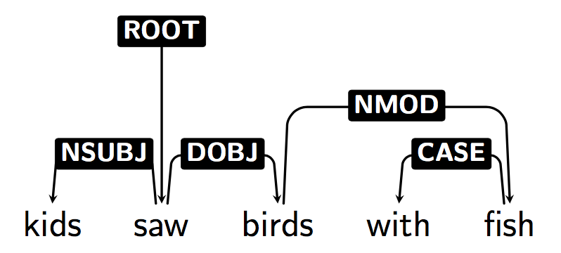
There is still disambiguation problem which vanilla PCFGs don't really solve.

• no lexical dependencies
  • e.g. "Kids saws birds with fish" vs "Kids saws birds with binoculars". PCFG yields the same parse tree when changing one word with another with the same POS tag.
  • fix: lexicaliztation
• no global structural preference
  • e.g. "Her dog bit her". 'her' should have different probabilities depending on where it occurs in the sentence.
  • fix: parent annotation

These fine grained grammar rules are specific but lead to huge grammar and sparse data.

Besides, constituent parsing is not good in complex environment such as other languages and domains.

Dependency syntax

Head dependent relation is shown as directed edges which point from heads to their dependents. Words in a sentence are connected with edges (often labeled).

• A single distinguished root
• All other words have exactly one incoming edge
• A unique edge from root to each other word

It's also a tree.

Compared with phrase structure(i.e. constituency, element of CFGs), dependency syntax has many advantage:

1. Sensible for word free order language.
2. Identify syntactic relation (e.g. the subjective of a sentence)
3. Dependency pairs make good features for classifiers
4. parsing can be fast

However, the assumption of asymmetric relation in dependency grammar is not always correct. For example, which is the head of "green eggs and ham"? eggs? or and?

Dependency annotation can be obtained by converting phrase structure annotation to dependencies:

1. find heads (head rules) -> Lexicalized Constituency Parse Tree
2. collapse chains of duplicate lexical heads -> Dependency Tree

Dependency parsing

The arc-standard approach is the algorithm for transition based dependency parsing. It's based on shift-reducer algorithm but has 3 actions: ($s_1, s_2$ are the top and second items on the stack respectively.)

• Shift: read next word w_i from input and push onto stack
• LeftArc: assign head-dependent relation $s_2 \leftarrow s_1$
• RightArc: assign head-dependent relation $s_2 \rightarrow s_1$

An example parsing of "Kim saw Sandy":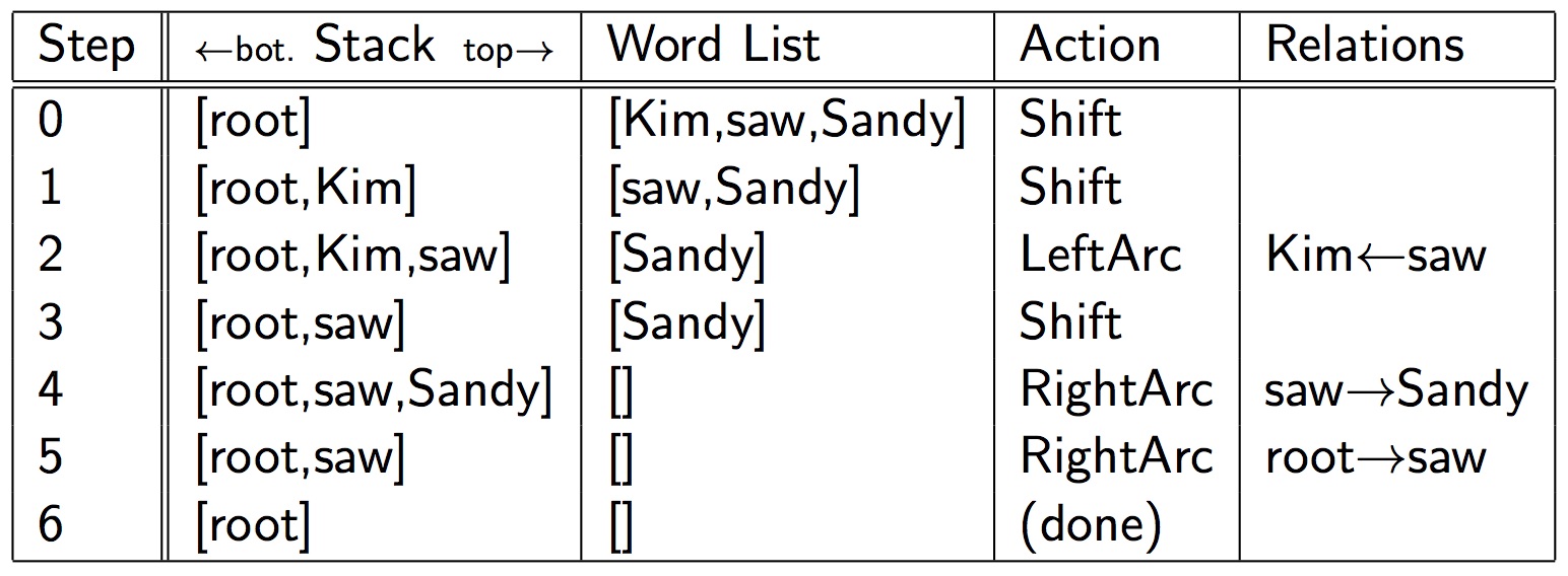

1. Greedy search: choose the most probable action at each step
   • time complexity is linear
   • The parse might not be the best one
2. Beam search: keep a fixed number of best actions rather than choose only the best action
   • More efficient than exhaustive search
   • more likely to find a better parse than greedy search

It must be pointed out that we need a good way to predict the correct action at each step, i.e. a logistic regression classifier which tells us P(action|configuration).

Dependency parsers are evaluated using the old accuracy: the proportion of the words where we predict correct heads (and label)

q 41: PCFG

Semantics

Currently, most AI systems are just mindlessly processing data. We want computers to understand the meaning instead.

Lexical semantics: meaning/sense of individual words

There are different relations between word senses.

• polysemy a word may have different meanings, e.g. interest
• synonymy different words have the same meaning, e.g. holiday vs vacation. antonymy is the opposite.
• hyponymy & hypernymy A is-a-kind-of B relationship, e.g. shark is a hyponym of animal
• meronymy part of, e.g. leg vs chair
• similarity similar in meaning, e.g. good vs great

WordNet is a hand-built ontology of synsets: sets of synonymous words. synets are connected by hyponym/hypernym, meronym, antonym relations. Polysemous words occur in multiple synsets.

word disambiguation

Given a polysemous word in a document and its possible senses (meanings), find which sense is intended.

This can be viewed as a classification task. Relevant features from sense labeled training data (e.g. SensEval) include

• neighboring words
• topic of document
• POS tag of target and surrounding words

Cons:

1. classifier must be trained separately for each word
2. require annotation for each word, useless for unseen or infrequent words

word similarity

Given 2 words, how similar are they?

Wordnet is not enough because it's not available for every language and some words might be missing. The methods discussed here can compute the similarity automatically.

According to distributional hypothesis, the meaning of a word can be inferred from the context it occurs in. This idea enables us to compute the similarity between 2 words automatically.

Distributional semantics (vector-space) models represent each word as a vector of its context words. Each dimension is a possible context word excluding stopwords. The corresponding value could be:

1. binary: either occurs (0) or not (1)
2. frequency
3. PMI
4. tf-idf

$$PMI(x, y) = \frac{P(x, y)}{P(x)P(y)}$$ PMI measures how much more/less likely two words occur together than if they are independent. In practice, probabilities are estimated by counts using MLE. It's sensitive to the incident co-occurrence of 2 low frequency words. There are 2 ways to better handle low frequencies: positive PMI or smoothing.

$$\begin{align} tf & = \log_{2} (1+f(t, d)) \\ idf & = \log_{2} (\frac{N}{n_t}) \\ tf-idf & = tf \cdot idf \end{align}$$

tf-idf is largely used in information retrieval to measure how important a word is to a document. Context words that are common everywhere have low scores.

Given context vectors for two words, how can we measure their similarity? Cosine is a good measure. Alternatives include Jaccard, Dice, Jenson-Shannon divergence

Intrinsic evaluation involves comparison with psycholinguistic data. For example, one can compute spearman rank correlation between 2 ranked lists of related words for a given word provided respectively by human judgement and the program.

dense representation 22

Both PPMI and tf-idf vectors are long (vocabulary size) and sparse (most of the elements are zero).

We might need short and dense vector representation because they

1. are easier to be included as features in machine learning algorithms
2. contain fewer parameters, generalize better and are less prone to overfitting
3. save memory

word embedding

Inspired by neural network, skip-grams (also referred to as word2vec) model trains a classifier to predict: Is a context word likely to show up near the given target word? The learned weights are word embeddings. The algorithm chooses surrounding context words as positive examples. For each positive context, the algorithm samples K non-neighbour words as negative context words. $$\log\sigma(c\cdot w) + \sum_{i=1}^{k} \log \sigma(-n_i \cdot w)$$ c is the positive context vector and $n_i$ are the vectors for K negative non-context words. $\sigma$ is a sigmoid function of the dot product and represents the similarity. Our goal is to learn vector representation of words to maximize the dot product of w and c and minimize the dot product of w and $n_i$.

The learning procedure (logistic regression) starts with randomly initialized vectors and iterates over the corpus to maximize this objective function.

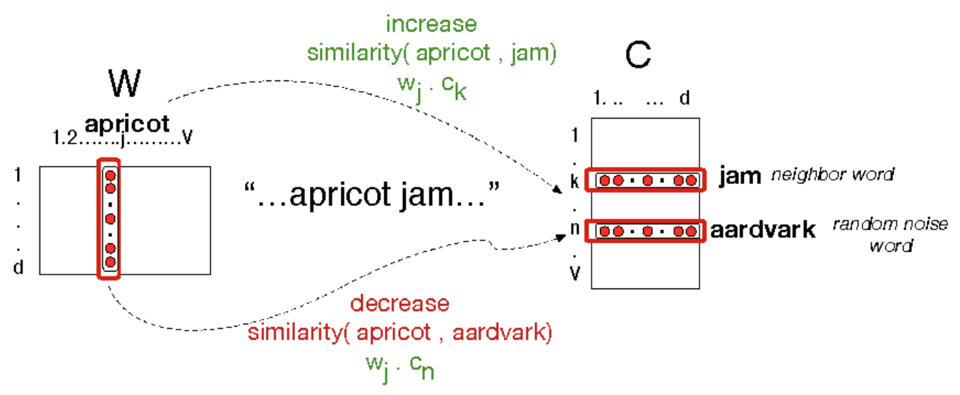
Each word has 2 embeddings, one in word matrix W and the other in context matrix C. There are some interesting properties about word embeddings. Offset between word embeddings can capture the relation between words. E.g. $vector(king) - vector(queen)$ is close to $vector(man) - vector(woman)$.

dimension reduction

Like PCA, Singular Value Decomposition (SVD) approximates an N dimensional dataset using fewer dimensions which capture the most variance in the original dataset. Latent Semantic Analysis (LSA) is a particular application of SVD to reduce the dimension of a term-document matrix representing |V| words and their co-occurrence with c documents (dimensions). Similarly, SVD can also be applied to word-word matrix or word-context matrix.

Sentence semantics

query: Did Poland reduce its carbon emissions?

facts/world/knowledge base:

• Carbon emissions have fallen for all countries in Central Europe.
• Poland is a country in Central Europe.

In order to deal with compositionally or inference, a machine needs to understand the sentence semantic.

Meaning representation

First, we need a symbolic and structured meaning representation language (MRL) to define the semantics.

MRL should have the following features:

1. compositional The meaning of a sentence is a function of its parts and rules by which they are combined.
2. verifiable The MR of a sentence can be used to determine whether the sentence is true with respect to some given model of the world.
3. unambiguous A MR corresponds to one interpretation. An ambiguous sentence should have a different MR for each meaning/sense.
4. canonical form Sentences with the same meaning should have the same MR, which simplifies inference and reduces storage.
5. inference We should be able to verify or answer from the MR of input sentence and facts in the knowledge base.
6. expressivity The MRL should allow us to handle a wide range of meanings in natural language and express appropriate relationships between the words in a sentence.

First order logic (FOL) is a kind of MRL. It consists of the following symbols:

1. constant, variable and function
   Constant denotes exactly one entity: John, 2018, this pen
   Variable ranges over entities: x
   Function denotes unique entity indirectly: father(John)

2. prediate
   Prediates with one argument represent property of entity. cat(Sam)
   Prediates with multiple arguments represent relations between entities. likes(John, Marie)
   A Predict followed by '/N' denotes a set of tuples (N arguments) that satisfy it. For example, like/N is the set of (x, y) pairs for which like(x, y) is true.
   Likewise, like(x, Maria) denotes the set of entities that like Maria.
   A prediate with one variable has a truth value if it's bond with a quantifier. e.g. ∀x.likes(x, cat)

3. logical connectives: ∨, ∧, ¬, ⇒
   For example, likes(Maria, John) ∧ tall(John) is true iff both prediates are true

4. quantifiers: ∀, ∃
   "Cats are mammals" has MR ∀x. cat(x) ⇒ mammal(x)
   "Maria owns a cat" has the MR ∃x. cat(x) ⇒ owns(Maria, x)
   "Everyone loves some movie" has 2 possible meanings (quantifier scope ambiguity):

   • ∃x. movie(x) ∧ ∀y. person(y) ⇒ loves(y, x)
   • ∀y. person(y) ⇒ ∃x. movie(x) ∧ loves(y, x)

FOL is a good match to natural language because

1. Arguments: nouns, NPs
2. Prediates: verbs, prepositions and adjectives
3. Logical connectives: coordination (or, and, not, if)
4. Quantifiers: determiners (a, an, any, every)

λ expression allows us to compute meaning representation compositionally.

λy. λx. love(x,y)(Jhon)(Maria) = λx. love(x,Maria)(Jhon) = love(Jhon, Maria)

John gave Mary a book
John gave Mary a book on Tuesday

A solution is to reify (to make concrete) events. The MR for the above 2 sentences are now:

∃ e, z. Giving(e) ∧ Giver(e, John) ∧ Givee(e, Mary) ∧ Given(e,z) ∧ Book(z)
∃ e, z. Giving(e) ∧ Giver(e, John) ∧ Givee(e, Mary) ∧ Given(e,z) ∧ Book(z) ∧ Time(e, Tuesday)

Semantic analysis

Given this way of representing meanings, how do we compute meaning representations from sentences?

Syntax driven semantic analysis rely on CGF rules with semantic attachment to build up the MR.

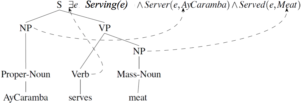
Rules with semantic attachments:

ProperNoun → AyCaramba  {AyCaramba}
  MassNoun → meat       {Meat}
        NP → ProperNoun {ProperNoun.sem}
        NP → MassNoun   {MassNoun.sem}
      Verb → serves     {λy. λx. ∃e. Serving(e) ∧ Server(e, x) ∧ Served(e, y)}
        VP → Verb NP    {Verb.sem(NP.sem)}
         S → NP VP      {VP.sem(NP.sem)}

So, the final semantic analysis of the sentences is

S.sem = VP.sem(NP.sem)
      = Verb.sem(NP.sem)(ProperNoun.sem)
      = λy. λx. ∃e. Serving(e) ∧ Server(e, x) ∧ Served(e, y)(Meat)(AyCaramba)
      = ∃e. Serving(e) ∧ Server(e, AyCaramba) ∧ Served(e, Meat)

Classifiers in NLP

1. naive bayes

   • Key feature: A generative model, model P(x, y) by assuming a generative process
   • Application: text/document categorization

2. logistic regression 18, 19

   • Key feature
     • A discriminative classifier, only model p(y|x) without generative process.
     • Avoid strong independence assumption
     • Can use arbitrary local and global features
     • Training is much slower
     • logistic regression can be viewed as a building block (a perceptron) of neural network.
   • Application: In NLP, multinomial logistic regression is also known as Maximum Entropy (MaxEnt)
     • word sense disambiguation (WSD)
     • dependency parsing: use MaxEnt to build model P(action|configuration). Features are various combinations of words and tags from stack and input.
     • n-best re-ranking: The first stage uses constituency parsing (generative) with beam search to output best n parses because it's fast to train and run. The second stage use MaxEnt model (discriminative) to rerank and pick the most probable parse because it can use arbitrary local/global features. The performance of the first stage is evaluated by oracle mechanism.

3. Multiple layer perceptron (MLP)

   • Key feature
     • Neural network contains one or more fully-connected hidden layers. Each node in a hidden layer applies a non-linear function of the weighted sum of its input and represents some learned feature
     • As a non-linear classifier, NN is more powerful than logistic regression
     • Vulnerable to local optima

Conclusion

NLP is an inter-disciplinary of linguistics and computer science. It allows us to solve many tasks in natural language using statistical or machine learning models with the help of linguistic theories.

• linguistics: build a better understanding of language structure
  • word, morphology, part of speech, syntactic, semantic
• computational methods
  • finite state machine (morphology analysis, POS tagging)
  • grammars parsing (CKY, statistical parsing)
  • probabilistic models and machine learning (HMMS, PCFG, Logistic regression, neural networks)
  • vector space (distributional semantics)
  • lambda expression (computational semantics)

Application of NLP

• information retrieval/extraction
• machine translation
• speech to text (Siri, Amazon echo)
• sentiment analysis

Language is hard to understand because of

• rules with exception
• ambiguity
• infinite